
8
Learning Objectives
- Calculate the limit of a function as
 increases or decreases without bound.
 - Recognize a horizontal asymptote on the graph of a function.
- Estimate the end behavior of a function as increases or decreases without bound.
- Recognize an oblique asymptote on the graph of a function.
To graph a function  defined on an unbounded domain, we also need to know the behavior of as
  In this section, we define limits at infinity and show how these limits affect the graph of a function.
Limits at Infinity
We begin by examining what it means for a function to have a finite limit at infinity. Then we study the idea of a function with an infinite limit at infinity. Back in Introduction to Functions and Graphs, we looked at vertical asymptotes; in this section we deal with horizontal and oblique asymptotes.
Limits at Infinity and Horizontal Asymptotes
Recall that  means
means  becomes arbitrarily close to
  as long as is sufficiently close to
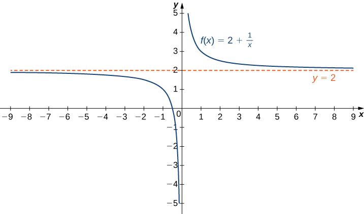
  We can extend this idea to limits at infinity. For example, consider the function
  As can be seen graphically in (Figure) and numerically in (Figure), as the values of get larger, the values of approach 2. We say the limit as approaches
  of is 2 and write
  Similarly, for
  as the values
  get larger, the values of approaches 2. We say the limit as approaches
  of is 2 and write
 as approaches
|
10 | 100 | 1,000 | 10,000 |
 |
2.1 | 2.01 | 2.001 | 2.0001 |
|
-10 | -100 | -1000 | -10,000 |
|
1.9 | 1.99 | 1.999 | 1.9999 |
More generally, for any function  we say the limit as
  of is if becomes arbitrarily close to as long as is sufficiently large. In that case, we write
  Similarly, we say the limit as
  of is if becomes arbitrarily close to as long as
  and is sufficiently large. In that case, we write
  We now look at the definition of a function having a limit at infinity.
Definition
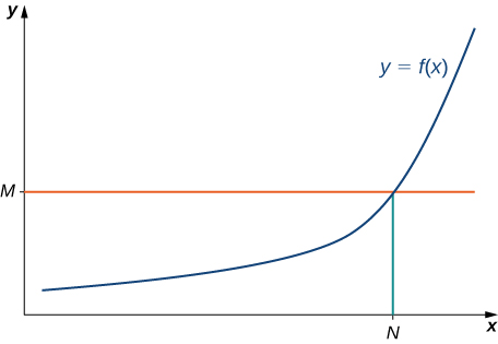
(Informal) If the values of become arbitrarily close to as becomes sufficiently large, we say the function has a limit at infinity and write

If the values of becomes arbitrarily close to for as becomes sufficiently large, we say that the function has a limit at negative infinity and write
If the values are getting arbitrarily close to some finite value as or  the graph of approaches the line
  In that case, the line
  is a horizontal asymptote of ((Figure)). For example, for the function
  since
since  the line
  is a horizontal asymptote of
Definition
If  or
or  we say the line is a horizontal asymptote of
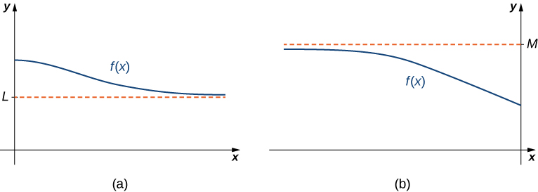
 the values of are getting arbitrarily close to
  The line is a horizontal asymptote of (b) As the values of are getting arbitrarily close to
  The line
  is a horizontal asymptote of
 A function cannot cross a vertical asymptote because the graph must approach infinity (or  from at least one direction as approaches the vertical asymptote. However, a function may cross a horizontal asymptote. In fact, a function may cross a horizontal asymptote an unlimited number of times. For example, the function
  shown in (Figure) intersects the horizontal asymptote
  an infinite number of times as it oscillates around the asymptote with ever-decreasing amplitude.
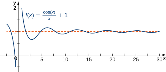
 crosses its horizontal asymptote an infinite number of times.
The algebraic limit laws and squeeze theorem we introduced in Introduction to Limits also apply to limits at infinity. We illustrate how to use these laws to compute several limits at infinity.
Computing Limits at Infinity
For each of the following functions evaluate  and
and  Determine the horizontal asymptote(s) for
Solution
- Using the algebraic limit laws, we have
 Similarly,
  Therefore,
  has a horizontal asymptote of
  and approaches this horizontal asymptote as
  as shown in the following graph.
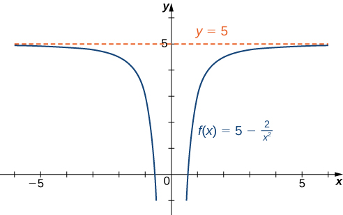
Figure 4. This function approaches a horizontal asymptote as - Since
 for all
  we have

for all
 Also, since
we can apply the squeeze theorem to conclude that

Similarly,

Thus,
 has a horizontal asymptote of and approaches this horizontal asymptote as as shown in the following graph.
Figure 5. This function crosses its horizontal asymptote multiple times. - To evaluate
 and
and  we first consider the graph of
  over the interval
  as shown in the following graph.
 The graph of
 has vertical asymptotes at
Since

it follows that

Similarly, since

it follows that

As a result,  and
and  are horizontal asymptotes of
  as shown in the following graph.
Evaluate  and
and  Determine the horizontal asymptotes of
  if any.
Hint

Solution
Both limits are 3. The line  is a horizontal asymptote.
Infinite Limits at Infinity
Sometimes the values of a function become arbitrarily large as (or as  In this case, we write
  (or
(or  On the other hand, if the values of are negative but become arbitrarily large in magnitude as (or as
  we write
  (or
(or 
For example, consider the function  As seen in (Figure) and (Figure), as the values become arbitrarily large. Therefore,
  On the other hand, as the values of
  are negative but become arbitrarily large in magnitude. Consequently,
|
10 | 20 | 50 | 100 | 1000 |
 |
1000 | 8000 | 125,000 | 1,000,000 | 1,000,000,000 |
|
-10 | -20 | -50 | -100 | -1000 |
|
-1000 | -8000 | -125,000 | -1,000,000 | -1,000,000,000 |
Definition
(Informal) We say a function has an infinite limit at infinity and write

if becomes arbitrarily large for sufficiently large. We say a function has a negative infinite limit at infinity and write

if  and
and  becomes arbitrarily large for sufficiently large. Similarly, we can define infinite limits as
Formal Definitions
Earlier, we used the terms arbitrarily close, arbitrarily large, and sufficiently large to define limits at infinity informally. Although these terms provide accurate descriptions of limits at infinity, they are not precise mathematically. Here are more formal definitions of limits at infinity. We then look at how to use these definitions to prove results involving limits at infinity.
Definition
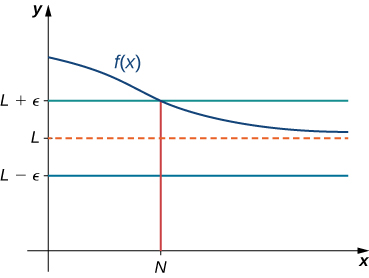
(Formal) We say a function has a limit at infinity, if there exists a real number such that for all  there exists
  such that

for all  In that case, we write
(see (Figure)).
We say a function has a limit at negative infinity if there exists a real number such that for all there exists  such that
for all  In that case, we write


Earlier in this section, we used graphical evidence in (Figure) and numerical evidence in (Figure) to conclude that  Here we use the formal definition of limit at infinity to prove this result rigorously.
A Finite Limit at Infinity Example
Use the formal definition of limit at infinity to prove that
Solution
Let  Let
Let  Therefore, for all we have

Use the formal definition of limit at infinity to prove that 
Hint
Let 
Solution
Let Let Therefore, for all we have

Therefore, 
We now turn our attention to a more precise definition for an infinite limit at infinity.
Definition
(Formal) We say a function has an infinite limit at infinity and write
if for all  there exists an such that

for all  (see (Figure)).
We say a function has a negative infinite limit at infinity and write
if for all  there exists an such that

for all
Similarly we can define limits as

Earlier, we used graphical evidence ((Figure)) and numerical evidence ((Figure)) to conclude that Here we use the formal definition of infinite limit at infinity to prove that result.
An Infinite Limit at Infinity
Use the formal definition of infinite limit at infinity to prove that
Solution
Let  Let
Let ![N=\sqrt[3]{M}.](https://opentextbooks.clemson.edu/app/uploads/quicklatex/quicklatex.com-5d31222eb8da1be538b8274beb5a60e8_l3.png "Rendered by QuickLaTeX.com") Then, for all we have
Then, for all we have
![{x}^{3} \symbol{"3E} {N}^{3}={(\sqrt[3]{M})}^{3}=M.](https://opentextbooks.clemson.edu/app/uploads/quicklatex/quicklatex.com-94db7a185bbfcfb410b216a649e6ee42_l3.png "Rendered by QuickLaTeX.com")
Therefore,
Use the formal definition of infinite limit at infinity to prove that 
Hint
Let 
Solution
Let Let Then, for all we have

End Behavior
The behavior of a function as  is called the function’s end behavior. At each of the function’s ends, the function could exhibit one of the following types of behavior:
- The function approaches a horizontal asymptote
- The function
 or
or 
- The function does not approach a finite limit, nor does it approach or
 In this case, the function may have some oscillatory behavior.
Let’s consider several classes of functions here and look at the different types of end behaviors for these functions.
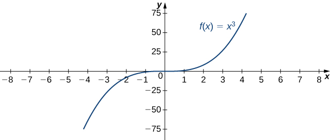
End Behavior for Polynomial Functions
Consider the power function  where
where  is a positive integer. From (Figure) and (Figure), we see that

and

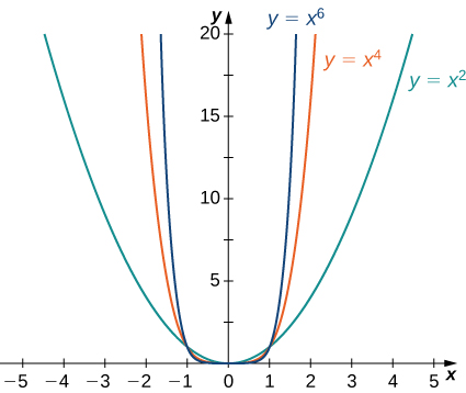


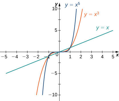
 and
and 
Using these facts, it is not difficult to evaluate  and
and  where
where  is any constant and is a positive integer. If
  the graph of
  is a vertical stretch or compression of
  and therefore

If  the graph of is a vertical stretch or compression combined with a reflection about the -axis, and therefore

If  in which case
Limits at Infinity for Power Functions
For each function evaluate and

Solution
- Since the coefficient of is -5, the graph of
 involves a vertical stretch and reflection of the graph of
  about the -axis. Therefore,
  and
and 
- Since the coefficient of
 is 2, the graph of
  is a vertical stretch of the graph of
  Therefore,
  and
and 
- This is an
 form so limit laws don’t help. However, by factoring we get
 As
As  , the power
  where the second factor gets close to
  . Hence the limit is
  As
As  , the power
  where the second factor gets close to . Hence the limit is
Let  Find
Find 
Hint
The coefficient -3 is negative.
Solution
End Behavior for Algebraic Functions
The end behavior for rational functions and functions involving radicals is a little more complicated than for polynomials. To evaluate the limits at infinity for a rational function, we divide the numerator and denominator by the highest power of appearing in the denominator. This determines which term in the overall expression dominates the behavior of the function at large values of 
Determining End Behavior for Rational Functions
For each of the following functions, determine the limits as and Then, use this information to describe the end behavior of the function.


Solution
- The highest power of in the denominator is Therefore, dividing the numerator and denominator by and applying the algebraic limit laws, we see that

Since
 we know that
  is a horizontal asymptote for this function as shown in the following graph.
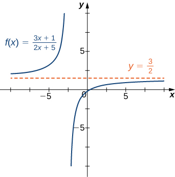
Figure 14. The graph of this rational function approaches a horizontal asymptote as - Since the largest power of appearing in the denominator is
 divide the numerator and denominator by
  After doing so and applying algebraic limit laws, we obtain

Therefore
has a horizontal asymptote of as shown in the following graph.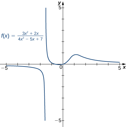
Figure 15. The graph of this rational function approaches the horizontal asymptote as - Dividing the numerator and denominator by we have

As
 the denominator approaches 1. As the numerator approaches
  As the numerator approaches Therefore
  whereas
  as shown in the following figure.
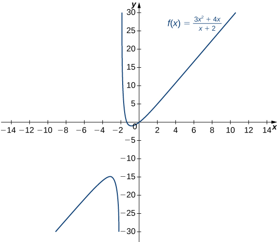
Figure 16. As the values  As the values
Evaluate  and use these limits to determine the end behavior of
Hint
Divide the numerator and denominator by 
Solution

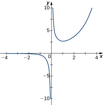
Before proceeding, consider the graph of  shown in (Figure). As and the graph of appears almost linear. Although is certainly not a linear function, we now investigate why the graph of seems to be approaching a linear function. First, using long division of polynomials, we can write

Since  as we conclude that

Therefore, the graph of approaches the line  as This line is known as an oblique asymptote for ((Figure)).
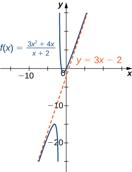
 approaches the oblique asymptote
Now let’s consider the end behavior for functions involving a radical.
Determining End Behavior for a Function Involving a Radical
Find the limits as and for  and describe the end behavior of
Solution
Let’s use the same strategy as we did for rational functions: divide the numerator and denominator by a power of To determine the appropriate power of consider the expression  in the denominator. Since

for large values of in effect appears just to the first power in the denominator. Therefore, we divide the numerator and denominator by  Then, using the fact that
  for
for 
 for and
  for all we calculate the limits as follows:

Therefore, approaches the horizontal asymptote as and the horizontal asymptote  as as shown in the following graph.
Evaluate 
Hint
Divide the numerator and denominator by
Solution

Determining End Behavior for Transcendental Functions
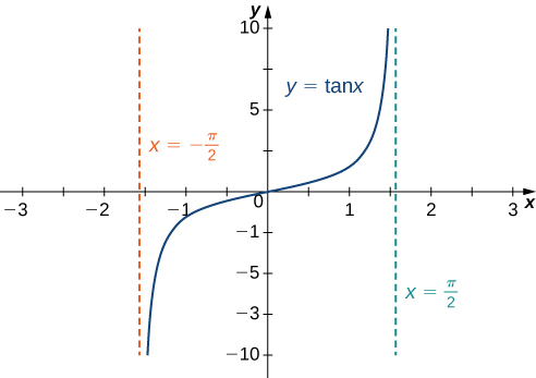
The six basic trigonometric functions are periodic and do not approach a finite limit as For example,  oscillates between
  ((Figure)). The tangent function has an infinite number of vertical asymptotes as
  therefore, it does not approach a finite limit nor does it approach
  as as shown in (Figure).
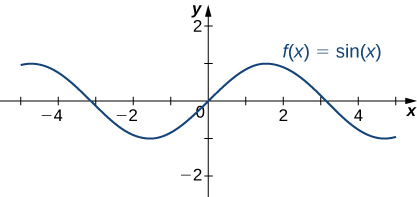
 oscillates between as
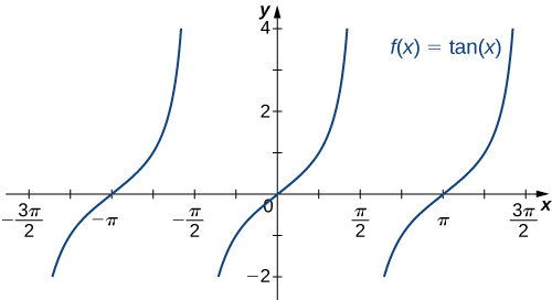
 does not approach a limit and does not approach as
 Recall that for any base  the function
  is an exponential function with domain
  and range
  If
If  is increasing over
  If
If  is decreasing over
  For the natural exponential function
 Therefore,
  is increasing on
  and the range is
  The exponential function approaches as and approaches 0 as as shown in (Figure) and (Figure).
|
-5 | -2 | 0 | 2 | 5 |
 |
0.00674 | 0.135 | 1 | 7.389 | 148.413 |
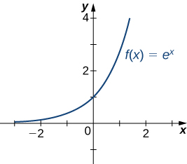 and approaches as
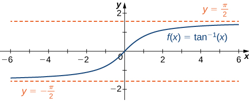
Recall that the natural logarithm function  is the inverse of the natural exponential function
  Therefore, the domain of is
  and the range is The graph of is the reflection of the graph of
  about the line
  Therefore,
  as
as  and
and  as as shown in (Figure) and (Figure).
|
0.01 | 0.1 | 1 | 10 | 100 |
 |
-4.605 | -2.303 | 0 | 2.303 | 4.605 |
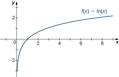 as
as Determining End Behavior for a Transcendental Function
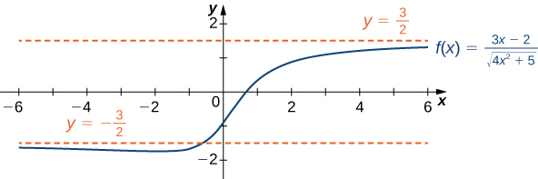
Find the limits as and for  and describe the end behavior of
Solution
To find the limit as divide the numerator and denominator by 

As shown in (Figure),  as Therefore,

We conclude that  and the graph of approaches the horizontal asymptote
  as To find the limit as use the fact that
  as to conclude that
  and therefore the graph of approaches the horizontal asymptote
  as
as
Find the limits as and for 
Hint
 and
and 
Solution
 ,
, 
Key Concepts
- The limit of is as (or as
 if the values become arbitrarily close to as becomes sufficiently large.
 - The limit of is as if becomes arbitrarily large as becomes sufficiently large. The limit of is as if and becomes arbitrarily large as becomes sufficiently large. We can define the limit of as approaches similarly.
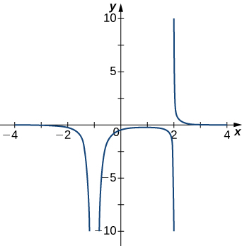
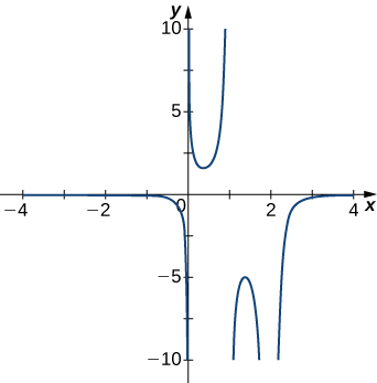
For the following exercises, examine the graphs. Identify where the vertical asymptotes are located.
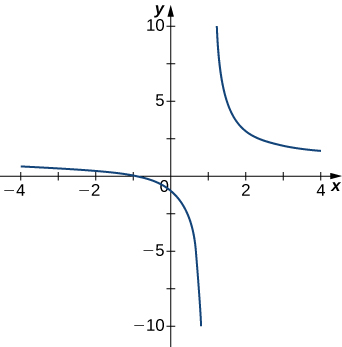
Solution

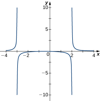
Solution

Solution

For the following functions  determine whether there is an asymptote at
  Justify your answer without graphing on a calculator.
6. 
7. 
Solution
Yes, there is a vertical asymptote
8. 
9. 
Solution
Yes, there is vertical asymptote
10. 
For the following exercises, evaluate the limit.
11. 
Solution
0
12. 
13. 
Solution
14. 
15. 
Solution

16. 
17. 
Solution
-2
18. 
19. 
Solution
-4
20. 
21. 
Solution

22. 
23. 
Solution

24. 
For the following exercises, find the horizontal and vertical asymptotes.
25. 
Solution
Horizontal: none, vertical:
26. 
27. 
Solution
Horizontal: none, vertical: 
28. 
29. 
Solution
Horizontal: none, vertical: none
30. 
31. 
Solution
Horizontal:  vertical:
32. 
33. 
Solution
Horizontal: vertical: and 
34. 
35. 
Solution
Horizontal:  vertical:
36. 
37. 
Solution
Horizontal: none, vertical: none
38. 
39. ![f(x) = \frac{x}{\sqrt[3]{x^3+1}}](https://opentextbooks.clemson.edu/app/uploads/quicklatex/quicklatex.com-0501857cd2954e10e4c13380b1834e1c_l3.png "Rendered by QuickLaTeX.com")
Solution
Horizontal:  , vertical:
40. 
For the following exercises, construct a function that has the given asymptotes.
41. and
Solution
Answers will vary, for example: 
42. and
43.  and
and
Solution
Answers will vary, for example: 
44.
For the following exercises, graph the function on a graphing calculator on the window ![x=\left[-5,5\right]](https://opentextbooks.clemson.edu/app/uploads/quicklatex/quicklatex.com-6570e421af5bd09e0ea47f2580908a9f_l3.png "Rendered by QuickLaTeX.com") and estimate the horizontal asymptote or limit. Then, calculate the actual horizontal asymptote or limit.
and estimate the horizontal asymptote or limit. Then, calculate the actual horizontal asymptote or limit.
45. [T]
Solution
46. [T]
47. [T]
Solution
48. [T]
49. [T]
Solution
50. True or false: Every ratio of polynomials has vertical asymptotes.
Glossary
- end behavior
- the behavior of a function as and
- horizontal asymptote
- if or then is a horizontal asymptote of
- infinite limit at infinity
- a function that becomes arbitrarily large as becomes large
- limit at infinity
- the limiting value, if it exists, of a function as or
- oblique asymptote
- the line
 if approaches it as or
