
4 Differential Kinematics
Rhyan Morgan
Differential Kinematics
4.1 The Analytical Jacobian
4.1 Angular Velocity and Linear Velocity
4.1.1 Pure Linear Velocity
4.1.2 Pure Angular Velocity
4.1.3 Relationship Between Linear and Angular Velocity
4.3 Geometric Derivation of the Jacobian
4.3.1 Skew Symmetric Matrices
4.3.2 Angular Velocity and the Skew Symmetric Matrix
4.3.3 Linear Velocity for the Geometric Jacobian
4.3.4 Deriving the Geometric Jacobian
4.4 Summary
Practice Questions
Simulation and Animation
References
Introduction
In Chapter 1, we have learned how to describe the orientation of a link with respect to (w.r.t.) a world or initial frame using the fundamental principles of rotation matrices. In addition, in Chapter 2, we have learned how to use the rotation matrices along with position information about a point in 3D space to formulate the homogeneous transformation matrix and derive the position and orientation of the end effectors of serial robot manipulators using principles of forward kinematics. Lastly, in Chapter 3, we have learned how to derive the inverse kinematics of a robot manipulator, i.e., the generalized coordinates of those series of joints to describe the overall configuration of the robot when the final position and orientation of the end effector are already known.
The information we have learned so far will be a foundation to the information presented in this chapter. In this chapter, we will learn how to describe the velocity of an end-effector given the velocities of its respective configuration of prismatic and revolute joints. We will describe the relationship between the angular and linear velocities of the end-effector and how they both play a role in the movement of the system. Neither can be disregarded as they are both important parts of the derivation process followed in this chapter.
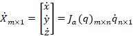
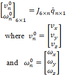
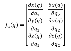
This chapter’s focus is the derivation of the Jacobian matrix which will relate the joint velocities to the end-effector velocity of a manipulator. Two different methods for attaining the Jacobian will be discussed, i.e, the analytical Jacobian and the geometric Jacobian. The Jacobian is a highly useful and important calculation in robotics. Many robotic motion planning and control algorithms depend on being able to derive the Jacobian. The analytical Jacobian will be introduced as the gradient of the forward kinematics. It will be an ![]() matrix where
matrix where ![]() represents the number of joints of the manipulator and
represents the number of joints of the manipulator and ![]() represents the degrees of freedom of the workspace.
represents the degrees of freedom of the workspace.
Then, angular and linear velocity will be explained, after which the derivation of the geometric Jacobian will be discussed. For a manipulator with ![]() links, the geometric Jacobian will be a
links, the geometric Jacobian will be a ![]() matrix that is directly multiplied by the
matrix that is directly multiplied by the ![]() matrix of joint velocities. This computation will output a
matrix of joint velocities. This computation will output a ![]() matrix of the respective linear and angular velocities of the end-effector. First, we will go over the derivation of the angular velocity and linear velocity Jacobians given by the orientation and position of the different joints of the manipulators. These two Jacobians can then be combined to produce the final
matrix of the respective linear and angular velocities of the end-effector. First, we will go over the derivation of the angular velocity and linear velocity Jacobians given by the orientation and position of the different joints of the manipulators. These two Jacobians can then be combined to produce the final ![]() geometric Jacobian. However, the result of this Jacobian is different from the analytical Jacobian. While the analytical and geometric Jacobians will have the same linear velocity terms, their angular velocity terms will differ. The analytical Jacobian relates the input velocities of the joints to Roll, Pitch, and Yaw rates, but the geometric Jacobian relates them to the angular velocities.
geometric Jacobian. However, the result of this Jacobian is different from the analytical Jacobian. While the analytical and geometric Jacobians will have the same linear velocity terms, their angular velocity terms will differ. The analytical Jacobian relates the input velocities of the joints to Roll, Pitch, and Yaw rates, but the geometric Jacobian relates them to the angular velocities.
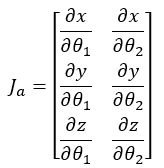
4.1 The Analytical Jacobian
The goal of this chapter is to figure out how the joint velocities affect the linear and angular velocities of the end-effector. The first method to discuss in solving for the velocities is the analytical Jacobian. Once the forward kinematics function, ![]() , is found, the analytical Jacobian is found by taking the partial derivative of each element of
, is found, the analytical Jacobian is found by taking the partial derivative of each element of ![]() w.r.t. each joint variable
w.r.t. each joint variable ![]() . In other words, the analytical Jacobian,
. In other words, the analytical Jacobian, ![]() , is the gradient of the function,
, is the gradient of the function, ![]() , w.r.t. each joint variable. This is shown in Equation (4.1).
, w.r.t. each joint variable. This is shown in Equation (4.1).
 |
(4.1) |
Since ![]() is a vector with
is a vector with ![]() inputs, one for each degree of freedom of the end-effector, the analytical Jacobian is
inputs, one for each degree of freedom of the end-effector, the analytical Jacobian is ![]() where
where ![]() represents the number of generalized coordinates (represented as
represents the number of generalized coordinates (represented as ![]() ) of the end-effector, or in other words, the number of joints. The analytical Jacobian of this form can then be multiplied by the generalized coordinate velocities, an
) of the end-effector, or in other words, the number of joints. The analytical Jacobian of this form can then be multiplied by the generalized coordinate velocities, an ![]() matrix represented as
matrix represented as ![]() , to obtain the velocity vector for the end-effector represented as
, to obtain the velocity vector for the end-effector represented as ![]() , which is shown in Equation (4.2).
, which is shown in Equation (4.2).
 |
(4.2) |
The analytical Jacobian can also help relate changes in roll, pitch, and yaw angles to angular velocity. The roll-pitch-yaw convention is one commonly used by engineers as well as pilots who use it to describe the orientation of aircraft.
Example 4.1.1
This example will show how to find the analytical Jacobian and end-effector velocity of a manipulator whose forward kinematics has already been found. The generalized coordinates of this example are ![]() and
and ![]() . The length
. The length ![]() is the distance from the revolute joint frame, {0}, to the first prismatic joint frame {1} and is not a generalized coordinate because it is held constant. This example uses the forward kinematics of a three-link cylindrical manipulator which are derived as Example 3.2 in the Robot Modeling and Control Textbook. (Spong, 2006)
is the distance from the revolute joint frame, {0}, to the first prismatic joint frame {1} and is not a generalized coordinate because it is held constant. This example uses the forward kinematics of a three-link cylindrical manipulator which are derived as Example 3.2 in the Robot Modeling and Control Textbook. (Spong, 2006)
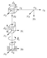 |
| Example Figure 1 Three-Link Cylindrical Robot (Spong, 2006) |
The forward kinematics matrix, ![]() is as follows (Spong, 2006):
is as follows (Spong, 2006):

Note that ![]() and
and ![]() represent
represent ![]() and
and ![]() respectively. The generalized coordinates of this example are
respectively. The generalized coordinates of this example are ![]() and
and ![]() . Therefore, when taking the gradient of
. Therefore, when taking the gradient of ![]() , it will be taken with respect to those variables.
, it will be taken with respect to those variables.
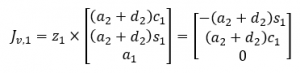
The first column of the analytical Jacobian will be the derivative of ![]() with respect to just
with respect to just ![]() , the second will be the derivative of
, the second will be the derivative of ![]() with respect to
with respect to ![]() , and the third will be the derivate of
, and the third will be the derivate of ![]() with respect to
with respect to ![]() . The result of these 3 calculations are shown:
. The result of these 3 calculations are shown:
 |
 |
 |
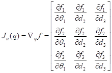
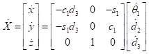
These 3 column vectors are then combined to create the following analytical Jacobian matrix:
 As equation 4.2.2 suggests, we can use this Jacobian to solve for the respective velocities of the end-effector as follows:
4.2 Angular Velocity and Linear Velocity
Angular and linear velocity of a rigid body are inherently related to each other. However, there are cases where a rigid body may experience purely linear velocity and purely angular velocity. These cases will be discussed as they bring some insight to why the two are related. These cases are generally rare in manipulators as there are usually several revolute and prismatic joints working together to create a specific motion or attain a specific position and orientation of the end-effector.
4.2.1 Pure Linear Velocity
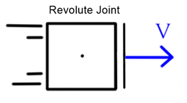
When a rigid body moves in a straight line and is not rotating, such as at the end of a simple prismatic joint, it will only have a linear velocity. At any instant, it will be moving a certain distance over a specified amount of time. As shown in Figure 4.1 a), since there is no rotation and since we assume the rigid body is moving in a straight line (rectilinear motion), there is no angular velocity. If the rigid body is moving on a curved path, but is still not rotating (curvilinear motion), as seen in Figure 4.1 b), the body itself also does not have an angular velocity associated with it, instead it will only have a linear velocity that is tangent to the path of travel. Note the differentiation between the body and the link in that with case b), the body is not rotating, but the link is.
 |
 |
| a) | b) |
Figure 4.1 Examples of block movements with pure linear motions: (a) block is moving in a straight path from a prismatic joint, and (b) block is moving in a curved path with no rotation.
When a rigid body’s movements are purely linear, such as in Fig. 4.1 a) and b), every point on that body will follow the same path of travel. This is obvious with case a), but can be seen in Fig. 4.1 b) as the green lines connect rigid points on the end effector as the object is moved through space. They each follow the same path as the red line indicating the path of travel of the center of the end-effector.
4.2.2 Pure Angular Velocity
When a rigid body rotates about a center of rotation (e.g., its center of mass) as shown in Fig. 4.2 it only has angular velocity. In other words, the position of a point on the body is moving in a circle about the point which the body rotates. At any instant, the angular velocity of the object is the time rate of change of the angle of the object to an axis of rotation. As opposed to Fig. 4.1 b) the path that each point on the rigid body follows will not be the same as any other point. This is because the radius of the circular path created by each point will depend on the distance of that point to the center of rotation.
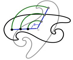 |
Figure 4.2 Pure rotation of a rigid body about point C by ![]() degrees. The initial orientation of the rigid body is shown in gray, and the orientation of the rigid body after rotation is shown in black.
degrees. The initial orientation of the rigid body is shown in gray, and the orientation of the rigid body after rotation is shown in black.
The case of pure rotation of a body can be seen in manipulators when the distance from one frame of reference to another is zero. A common example is a 3 degree-of-freedom wrist joint. Therefore, it is important to understand how the linear and angular velocities relate to each other for a rigid body that is not purely rotating about its center and is not simply translating.
4.2.3 Relationship Between Linear and Angular Velocity
In general, when a rigid body is moving in a curved path, with a linear tangential velocity, ![]() , it is also rotating with an angular velocity,
, it is also rotating with an angular velocity, ![]() . Mathematically,
. Mathematically, ![]() and
and ![]() are related by Equation (4.3).
are related by Equation (4.3).
| (4.3) |
In this equation, ![]() is a vector in the
is a vector in the ![]() direction with a magnitude of
direction with a magnitude of ![]() which is the time derivative of
which is the time derivative of ![]() . The vector
. The vector ![]() is perpendicular to
is perpendicular to ![]() and has a magnitude of the distance between the axis of rotation and the center of the rigid body. The cross product of these two vectors gives the vector
and has a magnitude of the distance between the axis of rotation and the center of the rigid body. The cross product of these two vectors gives the vector ![]() which is perpendicular to the directions of both vectors
which is perpendicular to the directions of both vectors ![]() and
and ![]() and represents the object’s tangential velocity. This is shown in Fig. 4.3.
and represents the object’s tangential velocity. This is shown in Fig. 4.3.
 |
| . |
Figure 4.3 Rigid object rotating about revolute joint along red path of travel. ![]() is perpendicular to
is perpendicular to ![]() and
and ![]()
When the vector ![]() ’s magnitude is zero, this represents pure rotation, and the tangential velocity will also be zero.
’s magnitude is zero, this represents pure rotation, and the tangential velocity will also be zero.
4.3 Geometric Derivation of the Jacobian
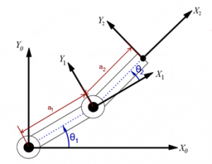
Once the relationship between the linear and angular velocities of a rigid body is established, we can move forward in understanding how to represent the total velocity of an end-effector of a manipulator. It is understood from Chapters 1 and 2 that the end effector’s instantaneous position is dependent on the instantaneous configuration of the preceding series of joints it is attached to. Each joint is either prismatic or revolute and has its own frame attached to it. If the joint is prismatic, its position is dependent on the extension of the joint. If the joint is revolute, the position and orientation are dependent on the length of the link it is attached to and the angle of rotation it is at. The angle of rotation is the generalized coordinate because it is the only changing variable when a simple revolute joint is actuated.
4.3.1 Skew Symmetric Matrices
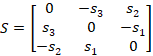
The skew symmetric matrix will be important as it has properties that make the derivation of the geometric Jacobian possible and simple. By definition, the skew symmetric matrix, ![]() is a square matrix such that adding the transpose to itself will be zero. This is seen as Equation (4.4).
is a square matrix such that adding the transpose to itself will be zero. This is seen as Equation (4.4).
| (4.4) |
This is possible only when all the diagonal terms of the matrix are zero and when the off-diagonal terms are inversed and the negative of each other. This is shown as Equation (4.5)
 |
(4.5) |
The 3×3 skew symmetric matrix is a convenient way to organize any 3-entry vector. For example, given the vector, ![]() , the skew symmetric matrix
, the skew symmetric matrix ![]() is shown as Equation (4.6).
is shown as Equation (4.6).
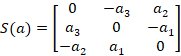 |
(4.6) |
The skew symmetric matrix operator, ![]() , uses the independent values of vector
, uses the independent values of vector ![]() and puts the entries in a form that has several unique and useful properties listed below.
and puts the entries in a form that has several unique and useful properties listed below.
- 1) The
 operator is linear so Equation (4.7) is true where
  and
and  are 3-entry vectors and
  are scalar. (Spong, 2006)
| (4.7) |
- 2) The cross product of two vectors, and , which have 3 entries each, is the same as the matrix multiplication of
 by . This is shown as Equation (4.8). (Spong, 2006)
| |
(4.8) |
- 3) Given a vector
 and a rotation transformation,
  , Equation (4.9) is true. (Spong, 2006)
| (4.9) |
- 4) For a skew symmetric matrix, , and a vector,
 , with appropriate length w.r.t. the dimensions of , Equation (4.10) is true. Note that for an
  skew symmetric matrix, has
  entries. (Spong, 2006)
| (4.10) |
4.3.2 Angular Velocity and the Skew Symmetric Matrix
It is shown in Chapter 4 of (Spong, 2006) that taking the derivative of a rotation matrix multiplied by its transpose and comparing the result to the requirements of a skew symmetric matrix, the following relationship can be derived as Equation (4.11)
| (4.11) |
It is also mentioned that with similar logic to the derivation of Equation (4.11), the following equation holds
| (4.12) |
In this expression, ![]() , represents the scalar angular velocity of the frame which the rotation matrix is related to. This expression is useful in taking the derivative of the rotation matrices which are used in robotics to find the position of a point,
, represents the scalar angular velocity of the frame which the rotation matrix is related to. This expression is useful in taking the derivative of the rotation matrices which are used in robotics to find the position of a point, ![]() , given relative to a fixed frame. With pure rotation, recall that to find the coordinates of a point
, given relative to a fixed frame. With pure rotation, recall that to find the coordinates of a point ![]() w.r.t. some fixed frame, one can multiply the rotation matrix from the fixed frame to the current frame of
w.r.t. some fixed frame, one can multiply the rotation matrix from the fixed frame to the current frame of ![]() by the coordinates of
by the coordinates of ![]() w.r.t. its current frame. Taking the derivative of the position of point
w.r.t. its current frame. Taking the derivative of the position of point ![]() w.r.t. the fixed frame, gives the point’s velocity, and from Equation (4.3), it is known that this velocity is equivalent to the angular velocity of the point crossed product with the vector representing the point in space.
w.r.t. the fixed frame, gives the point’s velocity, and from Equation (4.3), it is known that this velocity is equivalent to the angular velocity of the point crossed product with the vector representing the point in space.
To show that Equation (4.12) is using a skew symmetric matrix with values of angular velocity, the following succession of computations is taken starting with the equation to find point ![]() w.r.t. the fixed frame. (Spong, 2006)
w.r.t. the fixed frame. (Spong, 2006)
| (4.13) | |
| Step 1 is to take the derivative of both sides, and since |
|
| (4.14) | |
| The derivative of the position in frame {0} is the tangential velocity of the point. Therefore, the following is true: | |
| (4.15) | |
| Therefore, substituting (4.13) into (4.15) gives the following: | |
| (4.16) | |
| Finally, using the relationship defined by Equation (4.8), the cross-product can be rewritten as this: | |
| (4.17) | |
| Note that the result presented as (4.17), is the exact result if Equation (4.12) were used directly in (4.14) |
This is a general example of angular velocity, but with robotic manipulators, there are often multiple rotation matrices relating a point from a current frame to a fixed frame. So, how does one account for multiple input angular velocities from multiple frames? This is explained in Robot Modeling and Control, through a series of calculations involving the skew symmetric matrix operator, starting with the simple expression that a rotation matrix of a frame {2} w.r.t. frame {0} is the equivalent of the rotation matrix of frame {1} w.r.t. {0} multiplied by the rotation matrix of frame {2} w.r.t. frame {1}. In other words, we can start with Equation (4.18).
| (4.18) |
When the derivative of both sides is taken, the chain rule must be used and through the calculations and clever use of skew symmetric matrix properties represented by Equations (4.7) and (4.9), it is shown in the Modeling and Control text, that the angular velocity of frame {2} w.r.t. frame {0} is the same as the addition of the angular velocity of frame {1} w.r.t. frame {0} represented in frame {0} to the angular velocity of frame {2} w.r.t. frame {1} represented in frame {0}.
These calculations can be extended to multiple frames such that if ![]() represents the number of frames, Equation (4.18) is true. (Spong, 2006)
represents the number of frames, Equation (4.18) is true. (Spong, 2006)
| (4.18) |
Note that this equation uses the superscript to denote the representation frame, and the two subscripts are used to denote the frame of reference and the current frame.
4.3.3 Linear Velocity for the Geometric Jacobian
The rotation matrix relating the two frames is not enough to calculate the full geometric Jacobian because the rotation matrix only accounts for pure rotation of frames. Instead, the homogeneous matrix relating the two frames is used. Recall that the homogeneous matrix is of the form of Equation (4.19).
| (4.19) |
The position of point ![]() w.r.t. frame {0} can then be represented more generally as well as the result of Equation (4.20). (Spong, 2006)
w.r.t. frame {0} can then be represented more generally as well as the result of Equation (4.20). (Spong, 2006)
| (4.20) |
It can be shown from section 4.3.2 that taking the derivative of both sides will result in the angular velocity crossed product with the vector of point ![]() in {0}, added to the derivative of
in {0}, added to the derivative of ![]() , or in other words, the tangential velocity of the point added to the linear velocity of the frame the point is attached to.
, or in other words, the tangential velocity of the point added to the linear velocity of the frame the point is attached to.
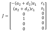
4.3.4 Deriving the Geometric Jacobian
As stated at the beginning of the chapter, the geometric Jacobian, ![]() , is a
, is a ![]() matrix that is multiplied by the generalized velocities of the
matrix that is multiplied by the generalized velocities of the ![]() joints that make up a robotic manipulator to attain the angular and linear velocities of the end-effector as shown in Equation (4.21).
joints that make up a robotic manipulator to attain the angular and linear velocities of the end-effector as shown in Equation (4.21).
 |
(4.21) |
As each manipulator can be assessed as a combination of prismatic and revolute joints, it is useful to calculate the Jacobian based on each joint individually.
For a prismatic joint, using the DH convention as introduced in Chapter 2, the actuation of the joint will result in a linear translation to the end-effector in the direction of the z-axis of the frame attached to that joint. If that joint is represented as ![]() , then the direction of the movement of the end-effector is in the
, then the direction of the movement of the end-effector is in the ![]() direction as shown in Fig. 4.4.
direction as shown in Fig. 4.4.
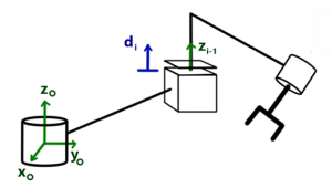 |
Figure 4.4 Prismatic joint geometric Jacobian representation
The velocity of the translation will have a magnitude of ![]() , which is the generalized velocity of joint
, which is the generalized velocity of joint ![]() . Once this is understood, Equation (4.22) can be used as the portion of the Jacobian relating to the linear velocity of that joint,
. Once this is understood, Equation (4.22) can be used as the portion of the Jacobian relating to the linear velocity of that joint, ![]() . Since there is no rotation in a prismatic joint, the rest of the Jacobian, i.e., the part relating to the angular velocity,
. Since there is no rotation in a prismatic joint, the rest of the Jacobian, i.e., the part relating to the angular velocity, ![]() , is zeros.
, is zeros.
|
Where |
(4.22) |
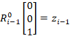
For a revolute joint, ![]() , the generalized velocity is
, the generalized velocity is ![]() which is about the
which is about the ![]() axis according to the DH convention. In this case, the angular velocity is obviously
axis according to the DH convention. In this case, the angular velocity is obviously ![]() . Taking the cross product of the angular velocity with the vector from the rotating frame to the end-effector will give the linear velocity of the end-effector due to the movement of the joint. The vector from the rotating frame to the end-effector is shown in Fig. 4.5.
. Taking the cross product of the angular velocity with the vector from the rotating frame to the end-effector will give the linear velocity of the end-effector due to the movement of the joint. The vector from the rotating frame to the end-effector is shown in Fig. 4.5.
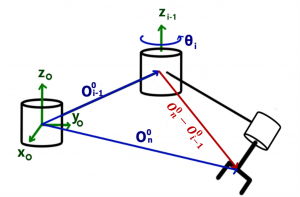 |
Figure 4.5 Revolute joint geometric Jacobian representation
Note that ![]() represents the position of the end-effector w.r.t. the fixed frame, and
represents the position of the end-effector w.r.t. the fixed frame, and ![]() represents the position of joint
represents the position of joint ![]() w.r.t. the fixed frame. Therefore, their difference represents the vector made from the end-effector to that joint. Hence, for a revolute joint, Equation (4.23) represents
w.r.t. the fixed frame. Therefore, their difference represents the vector made from the end-effector to that joint. Hence, for a revolute joint, Equation (4.23) represents ![]() w.r.t. a revolute joint.
w.r.t. a revolute joint.
| (4.23) |
Creating the full geometric Jacobian is simply a combination of the above derivations for ![]() and
and ![]() which can be found easily while only knowing the forward kinematics of the manipulator. To combine the values and create the Jacobian it is important to understand the Jacobian’s structure a bit more clearly. We know
which can be found easily while only knowing the forward kinematics of the manipulator. To combine the values and create the Jacobian it is important to understand the Jacobian’s structure a bit more clearly. We know ![]() is a
is a ![]() matrix where
matrix where ![]() is the number of joints used in the manipulator. The 6 rows are related directly to the 6 entries of the output velocity matrix that results from multiplying
is the number of joints used in the manipulator. The 6 rows are related directly to the 6 entries of the output velocity matrix that results from multiplying ![]() by the vector of joint velocities,
by the vector of joint velocities, ![]() . The top 3 entries relate to the
. The top 3 entries relate to the ![]() linear velocities, and the bottom 3 entries relate to the angular velocities, respectively. The
linear velocities, and the bottom 3 entries relate to the angular velocities, respectively. The ![]() column represents the Jacobian entries for the
column represents the Jacobian entries for the ![]() generalized coordinate velocity,
generalized coordinate velocity, ![]() . Therefore, given the information about prismatic and revolute joints, Table 4.1 can be utilized to derive the geometric Jacobian.
. Therefore, given the information about prismatic and revolute joints, Table 4.1 can be utilized to derive the geometric Jacobian.
Table 4.1 Geometric Jacobian Entries for Prismatic and Revolute Joints
| Jacobian Entries | Joint is Revolute | Joint is Prismatic |
| 0 |
The Jacobian’s full form is then created using Equation (4.24)
| (4.24) |
4.4 Summary
In Chapter 4, we covered the method for finding both the analytical and geometric Jacobians, where the only information we need about the manipulator is its forward kinematics. This is sufficient to finding the Jacobian, which can then be multiplied be a vector of the joint velocities of the manipulator to find the end-effectors linear and angular velocities. The analytical Jacobian is described by Equation (4.1) as simply the gradient of the forward kinematics function, ![]() , of the robotic system.
, of the robotic system.
Once the analytical Jacobian was derived, we covered the basics of angular and linear velocities in Section 4.2 as they relate to each other and are needed to understand the derivation of the geometric Jacobian in Section 4.3.
At the beginning of Section 4.3, we go over the skew-symmetric matrix, its operator, ![]() , and the four properties that make it unique and useful in deriving the geometric Jacobian. The operator, makes calculating the angular and linear velocities of an end-effector with respect to a reference frame simpler. Finally, after understanding the linear and angular velocity derivations, Table 4.1 is created and used along with Equation (4.24) to get the full
, and the four properties that make it unique and useful in deriving the geometric Jacobian. The operator, makes calculating the angular and linear velocities of an end-effector with respect to a reference frame simpler. Finally, after understanding the linear and angular velocity derivations, Table 4.1 is created and used along with Equation (4.24) to get the full ![]() geometric Jacobian.
geometric Jacobian.
While the results of the analytical vs. geometric Jacobian are very different from each other, they essentially have the same goal. They are used to represent the velocity of the end-effector of a manipulator when multiplied by a vector of generalized velocities. They reference different frames and have different looking results, but they are both useful in their common goal. As of now, this text has covered how to attain the forward kinematics, inverse kinematics and differential kinematics. Chapter 5 will build off these concepts and introduce dynamics.
Practice Questions
Calculating the partial derivatives gives the following as the final answer to problem 1.
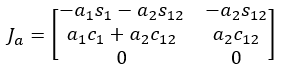
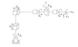 Diagram from Figure 3.9 of (Spong 2006)
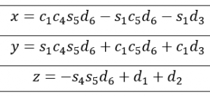
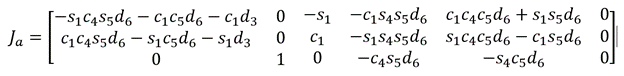
The analytical Jacobian is then found by taking the partial derivatives of the forward kinematics listed as the x, y, and z equations in the problem statement, with respect to each of the generalized coordinates. There are 3 terms in the forward kinematics and 6 generalized coordinates, therefore the analytical Jacobian will have 12 entries as shown:
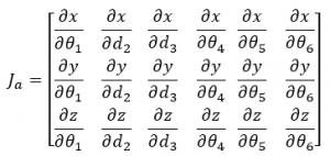
After computing the partial derivatives, the following is the final Analytical Jacobian:
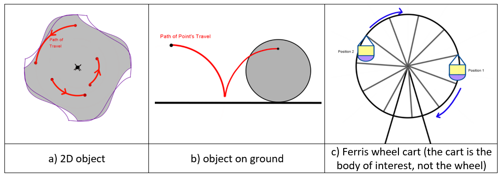
a. The object is moving with pure rotation. Because the path of travel of rigid points are not the same as each other, the body is not in pure linear motion. The paths have an arc shape with the center of the object as the center point of all 3 arcs shown, therefore the object is rotating about that point, and that center point itself is not moving, so there is no linear motion.
b. The object has rotational and angular velocities. The object can be seen as something round rolling on a flat surface. The arcs created by the point on the body do not create a perfect circle so the body is not purely rotating. If the object were in pure linear motion, the orientation of the object would stay the same and the point would not be able to get any closer to the ground. Therefore, the object is rotating and translating. It’s rotating about the center of the object, but that center is also moving along the path of the ground.
c. This body is in pure linear motion. A Ferris wheel itself rotates about its center point, but each individual cart must stay in the same orientation or risk the riders falling out of them. At the 1st position, the cart is upright, and at the second position, the cart is in the same orientation, meaning the cart does not rotate as it moves along the path of the Ferris wheel.
4. Find the geometric Jacobian for the following manipulator:
*Note that this is the same manipulator shown in chapter 2, example 6 and therefore has the same transformation matrixes and forward kinematics as follows:
Answer: We will start with finding the first column of the Jacobian which corresponds to the frame {0}. This frame is in line with the world frame, therefore:
The end effector position is given by the inverse kinematics and the frame {0} position is simply 0 from the world frame since they are coincident. Therefore:
The second joint is prismatic, so the bottom 3 values of its column of the Jacobian are all o. The to, is its z-axis transformed into the world frame which from the forward kinematics, is the following:
The final geometric Jacobian is:
Simulation and Animation

The simulation utilizing concepts of differential kinematics and comparing an approximation with a simulation of the Niryo One Robot shown below can be found on Github at:
https://github.com/ClemsonFall2021ME8930IntroRobotics-HRI/Ch4_DifferentialKinematics
Explanation of the simulation and the results are shown in the following video produced by the author of this chapter:
References
Spong, H. V. (2006). Robot Modeling and Control. John Wiley & Sons, Inc.
Wang, Yue (2021). ME 8930: Introduction to Robotics. Clemson University Course
