
8 Mobile Robot Navigation System
Cavender Holt
Chapter Outline
- 8.1 Introduction
- 8.2 Sensors in Navigation
- 8.2.1 Lidar
- 8.2.2 Beacon
- 8.2.3 Compass
- 8.2.4 Odometry
- 8.2.5 Sonar
- 8.2.6 Camera
- 8.2.7 Sensor Fusion
- 8.3 Methods in Navigation
- 8.3.1 Line Following
- 8.3.2 Fuzzy Logic based Navigation Approach
- 8.3.3 Neural Network Controller based Navigation Approach
- 8.3.4 Soft Computing
- 8.3.5 SLAM Algorithms
- 8.3.6 Vector Filed Histogram
- 8.4 Summary
8.1 Introduction
Intelligent robots are required to perform tasks in domains such as space exploration, manufacturing in industry, military applications, and rescue during emergencies. Mobile robots are often employed in these environments as a large range must be covered to complete tasks such as transporting materials, searching for trapped individuals in hazardous environments, or exploring the surface of new planets. While mobile robots have excellent range, they are often deployed in complex environments that are difficult to navigate due to obstacles and harsh terrain. Since these mobile robots are expected to operate autonomously, mechanisms must be employed for the robot to understand its environment, determine the optimal path to reach the destination, and avoid obstacles within the environment. Additionally, when considering that these environments may be dynamic and constantly changing, the navigation mechanisms must be deployed on the robot since the environment cannot be determined before the robot traverses it. Researchers have developed multiple methodologies in order to tackle this problem throughout the years. The remainder of this chapter will discuss a survey of navigation methods used in robotics, sensors used to detect the surrounding environment and robot orientation, and behavior-based navigation.
In Chapter 7, we explored methods that allow a robot to generate a path that can be followed in space from a starting point to a goal point. These methods are often performed in a global scope and are prepared in an offline fashion. Additionally, they are often performed with a coarse granular knowledge about the specific obstacles and details of the region. Chapter 6 explored trajectory techniques and generation methods for a manipulator robot which defines how the joints move to reach a target point. We further explore problem areas in motion planning for when a mobile robot is deployed into relatively unknown environments. When a mobile robot is deployed, it is very important to have the ability to update the path in real-time at a local scale to avoid obstacles that were not known during the global path planning period. This chapter gives a survey of several methods to update the path locally to avoid obstacles and uncertainty in an environment. While many more techniques exist, we present a sample of popular methods and refer the reader to further explore this problem area in more detail after reading this section.
8.2 Sensors for Navigation
8.2.1 Lidar
Light Detection and Ranging (Lidar) is a common sensor that is used for mobile robotics in order to navigate dynamic environments. Lidar dynamically determines the distances from objects to the sensor by using lasers. The Lidar sensor shoots a laser beam outwards and then measures the amount of time it takes for the beam of light to return from reflecting off of the object. By sending out many of the lasers in a short period of time, the robotic system can create a map of depths from the surrounding environment in order to assist with navigation. One major component of a Lidar system is the laser which often ranges from 600-1000nm wavelengths. Another important component is phased arrays which may contain up to a million optical antennas in order to see the radiation pattern in a certain size and in a certain direction. Microelectromechanical machines are also used in order to allow one laser to be shot anywhere in the target field around the robotic system.
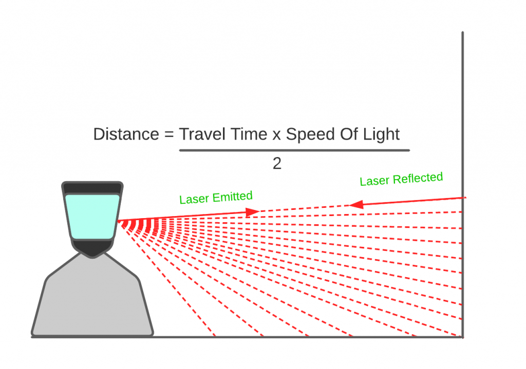
Figure 8.1: Lidar example function
8.2.2 Beacon
Beacon sensor systems are most often employed for mobile robotic systems in indoor environments. This is due to the fact the beacons must be fixed points of reference in the mobile robot’s coordinate frame. The beacons then emit a signal which allows a robot to determine its distance from the beacon. In order to obtain an accurate measure of the position of the robot in the plane, three beacons are needed. Each beacon emits its signal in a circle which gives the requirement of three beacons seen from Figure 8.2.
![]()
Figure 8.2: Beacon Intersection Constraints
8.2.3 Compass
A compass sensor is very useful for mobile robotics since they often travel fairly large amounts of distance. The compass sensor allows the robot to maintain a reference with regard to direction. Since the compass sensor will always know where north is due to the magnetic fields of the earth, it can use the direction as a reference in order to determine the current direction it is traveling. This is very useful in order to accurately follow paths that are planned from low-resolution data of the environment, and correction on the local level is needed. While this is one of the more straightforward sensors, often just using hall effects sensors, they are very impactful to mobile robotics.
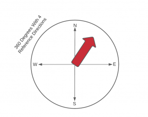
Figure 8.3: Compass Depiction
8.2.4 Odometry
Odometry is a method to measure the distance that a robot has traveled from its starting location. It is often a useful metric for mobile robots to know how far they have traveled in a given direction and the orientation the robot is currently in. In environments that are not super dynamic, mobile robots can use this sensor in particular because the distances that robots will have to travel are far more standardized. For example, a robot in a warehouse may have to follow a set path, and odometry could be primarily used to know how far a mobile robot must travel in a given direction before turning. One of the most common ways odometry systems are built is by using rotary encoders on the wheels of a mobile robotic system. Since the circumference of the wheels is known for a given robot, the system knows how much distance has been traveled through one rotation of the wheel. A rotary encoder subdivides a circle, and then the distance from each tick of the rotary encoder can be calculated from the circumference. Additionally, the position and orientation of the robot can be determined through the use of the rotary encoder ticks of each wheel and the standard mobile robot forward kinematics equations. One performance issue of this method is related to the fact that the accuracy of the distance is determined by the number of times the circle is subdivided. For example, if a rotary encoder only had four subdivisions, there is a large amount of distance between each time the distance is updated when rotating. Additionally, mechanical imperfections and improper sensors readings can cause an incorrect count of ticks that don’t correspond with the actual distance rotated. The distance that the wheel has rotated can be calculated by the Equation (8.1) where [latex]D_r[/latex] is the distance rotated, [latex]R[/latex] describes the radial distance from the center of the wheel, and [latex]\phi_r[/latex] is the angle that the wheel has rotated.
| [latex]D_r = R * \phi_r[/latex] | (8.1) |

Figure 8.4: Rotary encoder disk where each sector has a different code and therefore indicates a tick has been rotated.
8.2.5 Sonar
Sonar sensors are often employed in mobile robotic applications as they are similar to lidar sensors. They also provide information about distances to objects in the environment. The primary difference between these sensors is that Sonar uses sound in order to measure distance. In most sonar systems, a transducer sends out a sound wave at a frequency that is above the range of human hearing or 20kHz. This sound wave travels outward into the environment, and the sensor begins measuring the amount of time and will continue measuring the time until the wave bounces off of an object in the environment and returns to the sensor. The distance can be calculated by using the speed of sound and the time that was measured by the formula in Equation (8.2), where [latex]s[/latex] is the speed of sound, [latex]t[/latex] is time, and [latex]d[/latex] is the distance. This sensor allows the robot to understand the distance to obstacles surrounding it so it can make local navigation decisions.
| [latex]d = (s * t) / 2[/latex] | (8.2) |
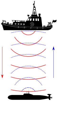 Figure 8.5: Sonar Functionality Example
8.2.6 Camera
A camera is also an essential tool used in mobile robotics in order to detail details about the local environment during navigation. While this type of sensor cannot be used to provide precision measurements to obstacles that surround the robot, it is still a useful sensor. In particular, a camera sensor can collect video frames of the environment which can be used for applications such as object detection. This can be useful to determine when certain objects exist around a robot, such as a pedestrian or an animal. A camera can also be used in applications such as line following or object detection in environments that have less certainty. The frame captured by the camera can be processed to look for certain colors that indicate certain actions to the robot. For example, if a robot encounters an orange line on the floor, it may reduce its speed or rotate. The performance of the camera as a sensor is impacted by conditions, environmental conditions such as lighting, and properties of data collection such as resolution. In general, the higher the resolution, the more accurate the information provided by the image frame.
8.2.7 Sensor Fusion
Sensor fusion is the process of combining multiple sensor sources in order to remove uncertainty from the measurements taken to inform the robot how it should navigate a given space. An example of this may be when a robot is trying to determine its location in a coordinate system. By combining signals from sensors such as a camera and Lidar, the robot may be able to more accurately determine its current position than by using the two sensors independently of each other. There are several common methodologies in order to fuse together sensors, the first of which is inverse variance weighting. Suppose we have measurements of two sensors denoted by the variables [latex]Y_1[/latex] and [latex]Y_2[/latex], and each sensor variable has an associated noise variance given by [latex]\omicron_1[/latex] and [latex]\omicron_2[/latex]. The measurement for the combination of the two sensors can be given by Equations (8.3 and 8.4). These equations show that the fused measurement is a linear combination of the two sensors weighted by the variances associated with each sensor.
| [latex]Y_3 = \omicron_3^2 ( \omicron_1^{-2} * Y_1 + \omicron_2^{-2} * Y_2 )[/latex] | (8.3) | |
| [latex]\omicron_3^{2} = (\omicron_1^{-2} + \omicron_2^{-2})^{-1}[/latex] | (8.4) |
A second methodology to fuse sensors is to use an optimal Kalman Filter. The Kalman Filter is used to estimate states of linear dynamic systems within the state space. The process model and the measurement model are defined by Equations (8.5 and 8.6).
| [latex]x_k = Fx_{k-1} + Bu_{k-1} + w_{k-1}[/latex] | (8.5) | |
| [latex]z_k = Hx_k + v_k[/latex] | (8.6) |
Where [latex]F[/latex] is the state transition matrix, [latex]x_k[/latex] and [latex]x_{k-1}[/latex] are the state vectors, [latex]B[/latex] is the control input matrix, [latex]u_k[/latex] is the control vector, and [latex]w[/latex] is the process noise vector. In the Equation (8.6), [latex]H[/latex] is the measurement matrix, [latex]v_k[/latex] is the measurement noise, and [latex]z_k[/latex] is the measurement vector. When applied to sensor fusion, Kalman Filters are used in four primary setups. The first method is the prefiltering method that filters the measurement signals before they are compared in order to determine the best estimate from the combined sensors. The second methodology applies the total states from the sensors and combines them together before they are filtered by the Kalman Filter to determine the best estimate. One disadvantage of this method is that the user must understand the dynamic model of the sensor in order to find the predicted position. This method is often called the total state space extended Kalman Filter. The last two methods are similar except that one performs feedforward with the estimation error, and the other performs feedback. The indirect feedforward Kalman Filter feeds the estimation error forward into a measured signal before the comparison is made. The indirect feedback Kalman Filter feeds the estimation error back into the measured signal before the comparison is made. Diagrams for these methods can be seen in Figure 8.6.
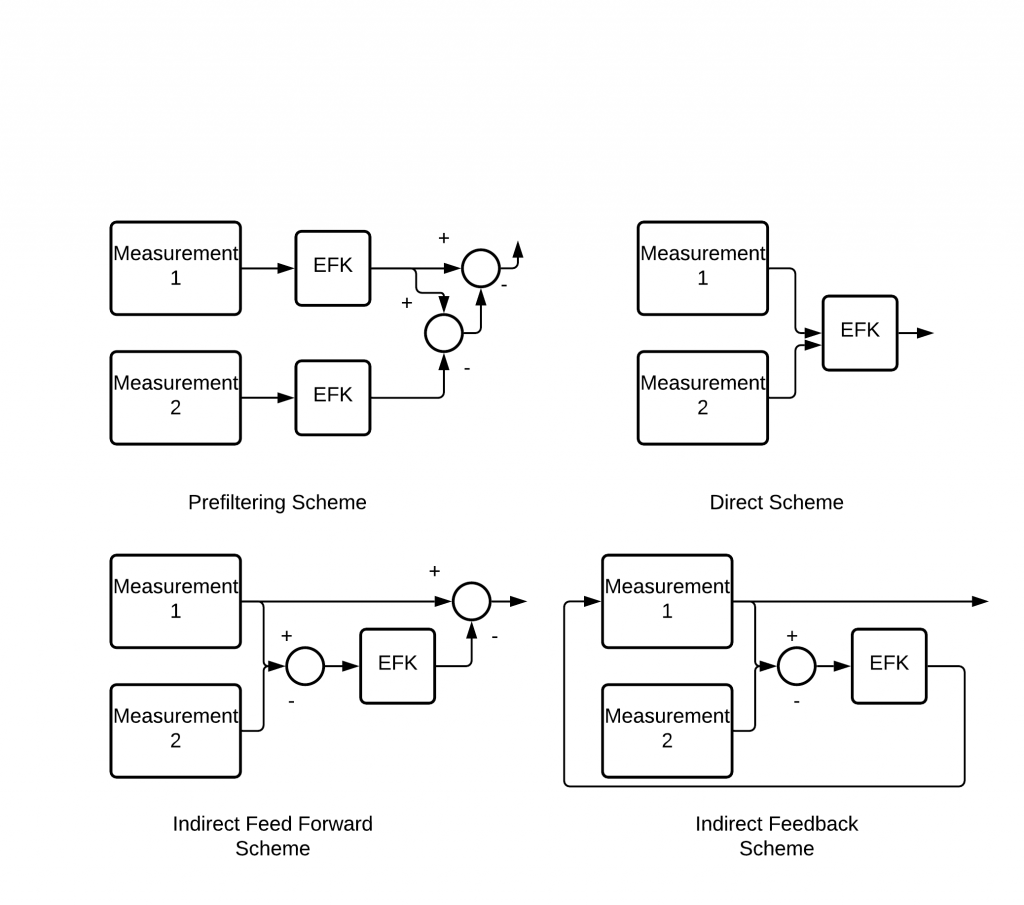
Figure 8.6: Diagrams for Kalman filter setups
8.3 Methods in Navigation
8.3.1 Line Following
Navigation by line following is one of the simpler forms of mobile robot navigation, but it has more limitations than methods discussed in 8.3.2 and 8.3.3. In particular, line-following navigation systems cannot be deployed in dynamic environments. Instead, line following systems are far more useful when deployed in environments such as warehouses or other industrial settings that are less dynamic than outdoor environments. In less dynamic environments, the lines can all be laid down such that the robots in the environment can follow the predetermined paths without issues. However, other systems may often be used to assist line following in case a moving obstacle crosses the line on which the robot is traveling to prevent collisions.
Most line following systems are built using infrared sensors deployed on the chassis of the robot. A line is painted on the floor that is a distinct color from the rest of the environment. The infrared sensor emits light that is reflected off the color on the floor. The amount of reflected light varies based on the color painted on the floor, and that change can be detected by the infrared receiver. Using this method allows the robot to understand when it begins deviating from the line that it should be traveling along. When the deviation begins to occur, control inputs can be generated in order to realign the robot to the line and continue onward following the correct path.
8.3.2 Fuzzy Logic-based Navigation Approach
Fuzzy logic is well suited to mobile robot control due to the uncertainty that exists in the environments in which mobile robots are deployed. In classical computing systems, boolean logic is applied to determine the state of a variable. An example of this would be a variable to define if a surface is cold. With boolean logic, the only values that we may apply to this variable are true or false. However, in reality, many would translate the state of the cold variable into more values such as very cold, sort of cold, not very cold, or not cold at all. This extra partitioning allows us to better understand the uncertainty in determining the temperature of a surface. This is where fuzzy logic can be deployed in order to combat uncertainty. Fuzzy logic defines multiple states that an input variable may take on, and then the probability that the input should take on that state is defined in the range 0 to 1. In order to determine if the input value belongs to a certain set, a membership function is created. If the membership function takes on the value of zero for a given input, the input does not belong to that set at all. If the membership function takes on a value of one, the input belongs completely to that set. A value between zero to one indicates partial membership to the set. An input value will take choose membership to the set with the highest value of its membership function. Fuzzy logic uses linguistic variables to represent rules and facts within the system. For example, a linguistic variable age may contain classes such as very young, young, old, and very old, representing the values that age may take on. An example of a membership function describing temperature can be seen below.
 Figure 8.7: Fuzzy logic membership function for a given input variable. A higher value indicates a stronger membership.
[latex]null[/latex]As seen in Figure 8.7, the temperature variable has five membership functions that it may belong to, ranging from cold to hot across a temperature range. This allows us to represent the concept of temperature at a finer granularity than true or false.
In general, fuzzy systems have three primary stages. The first stage takes the inputs to the system and fuzzifies them by using the membership functions that have been discussed previously. Applications then apply a set of If-Then rules to map to classes within the output variables. The final stage is to then map the output values back into a clear, concise signal that can be expressed as a physical value. We will now apply an example fuzzy system to the domain of mobile robotics, as shown in Figure 8.8. Suppose we have a variable called distance to an obstacle which gives the distance in feet before a mobile robot may collide with an obstacle. We can map this input using fuzzy logic to the sets very close, close, far, and very far. A membership function like the one below may then be created to map distance values to the correct classification. We can then use a set of If-Then rules to determine how the output variables, which we define as Right Wheel Velocity and Left Wheel Velocity, should be mapped to the input variable sets. We give the output variables sets of slow, medium, and fast. It is important to note that in this simple example, the robot can only perform several simple operations. The robot can rotate left quickly to turn, rotate left slowly to turn, drive forward slowly, and drive forward quickly.
IF very close THEN leftWheelVelocity fast AND rightWheelVelocity slow
IF close THEN leftWheelVelocity fast AND rightWheelVelocity medium
IF far THEN leftWheelVelocity medium AND rightWheelVelocity medium
IF very far THEN leftWheelVelocity fast AND rightWheelVelocity fast
Figure 8.8: Example If-Then Statements Mapping Input Fuzzy Sets to Output Fuzzy Sets
These output sets can then be mapped back to a crisp value that can control the speed of the motor based on the class of the output value.
8.3.3 Neural Network Controller Based Navigation Approach
Neural network controllers are also useful in assisting a robot in navigating complex dynamic environments. Training can be performed on likely scenarios that the mobile robot might encounter in an environment, and the correct control inputs that should be output when the scenario is encountered can be predicted. Additionally, during deployment, the mobile robot can continue training its model to make improvements based on the environment that it is deployed into. A set of sensors is often deployed on the robot to collect information about the surroundings of the robot, such as sonar sensors, cameras, lidar sensors, and odometry sensors.
A neural network is constructed of multiple layers of nodes. In particular, there is an input layer and an output layer that accepts inputs from a set of sensors, and the output is often connected to control inputs for some system. The hidden layers control the connection between input and output by storing weights between the nodes. As training is performed, the weights in the hidden nodes are updated such that the correct outputs are activated when a certain input sequence is seen. In particular, each node may be thought of as its own linear regression model, and each node contains a threshold value, a weight value, a bias value, and an output. Equation (8.7) shows how the output for a given node is calculated where [latex]W_i[/latex] represents that weight assigned to input from a previous node. The value [latex]X_i[/latex] represents the input value from a previous node, and B gives a bias that can be assigned to improve learning by shifting the activation function. The activation function is used to concisely map whether a node should be activated and is often represented by a sigmoid function. The variable [latex]Y_1[/latex] represents the output of a given node within the network. The input layer has its values multiplied by the weights connected to the node, and then the bias value is added. If this sum surpasses the activation threshold value, the output is passed to the next layer. An example neural network architecture can be seen in Figure 8.9.
| [latex]Y_1 = activation(W_1 * X_1 + W_2 * X_2 + W_3 * X_3 + B)[/latex] | (8.7) |

Figure 8.9: Fully connected neural network with 4 total layers. The input and output layers have two nodes each, and there are two hidden layers.
The neural network above takes two inputs, and in the domain of robotics, we could consider the first input to be the distance to an obstacle in front of the robot and the second input to be the distance to an obstacle on the left or right. The two outputs may indicate values such as move forward or turn. The training data may be constructed in a vector as follows [latex][x_{fb}, x_{lr}, o_{mf}, o_{t} ][/latex] where [latex]x_{fb}[/latex] is the distance to an obstacle in front or rear, [latex]x_{lf}[/latex] is an obstacle to the left or the right, and [latex]o_{mf}[/latex] is the output to move forward and [latex]o_{t}[/latex] is the output to turn the robot. By training this model, it will correctly predict the movement that it should perform given a set of inputs, allowing it to navigate correctly in dynamic systems.
8.2.4 SLAM Algorithms
SLAM or Simultaneous Localization and Mapping is an algorithm that continuously updates an environment map while maintaining the position of a robot within the map. Given a series of control inputs [latex]u_t[/latex] and a set of observations over a set of time steps [latex]t[/latex] , the SLAM algorithm must compute the robot position [latex]x_t[/latex] and compute a map of the environment [latex]m_t[/latex] . The general probabilistic equation for updating the map and location is given by Equations (8.8 and 8.9).
| [latex]P(m_t | x_t, o_{1:t},u_{1:t}) = \sum_{x_t} \sum_{m_t} P(m_t | x_t,m_{t-1}, o_{t},u_{1:t})P(m_{t-1},x_t | o_{1:t-1},m_{t-1},u_{1:t})[/latex] | (8.8) | |
| [latex]P(x_t | o_{1:t},u_{1:t},m_t) = \sum_{m_{t-1}} P(o_t | x_t,m_{t}, u_{1:t}) \sum_{x_{t-1}} P(x_t | x_{t-1})P(x_{t-1}| m_t,o_{1:t-1},u_{1:t})/Z[/latex] | (8.9) |
The overall slam process is composed of several steps, and as mentioned previously, the goal of the process is to update the map of the robot’s surroundings and update the position of the robot within that map. One of the most common tools used within SLAM is the lidar sensor introduced in section 8.2.1 due to its high precision measurements though it is often combined with another sensor such as odometry, which provides the general location while the lidar sensor provides correction to the odometry error. The lidar correction is performed by extracting features that have been mapped within the environment that are then reobserved by the robot. An Extended Kalman Filter (EKF) is the primary mechanism used to track not only the uncertainty in the robot’s current position but also the uncertainty of the features that have been mapped by the sensors as well. The high-level workflow for the SLAM algorithm starts when odometry observes an update indicating that the position of the robot has changed. The EKF updates the uncertainty of the position of the robot because it has moved. A lidar scan is then used to extract the features in the environment around the robot in its new position. The robot attempts to determine which of the observations from the current environment have already been seen and can be used to better update its current position. Observations of features that have not yet been seen are added to the EKF as new observations so that their information can be reused at a later time. This workflow repeats over and over as the robot explores a new environment. While the overall workflow remains largely the same, the tools by which the techniques are performed can be swapped, such as replacing lidar with a sonar sensor or by using point cloud registration instead of an EKF. SLAM algorithms are still widely researched, so the tools used often change and allow for novel additions, but the high-level problem and general process remain the same.
8.2.5 Vector Filed Histogram
The Vector File Histogram navigation technique utilizes histogram grids and polar histograms in order to determine the correct control inputs to avoid obstacles in an environment. The first step of the algorithm is to construct the histogram grid. The values in each cell of the histogram grid represent the obstacle vector at that location. The magnitude of the obstacle vector can be calculated by Equation (8.10). In the equation, [latex]a[/latex] and [latex]b[/latex] are given constants greater than zero. The variable [latex]c_{ij}^*[/latex] is a constant ranging from 0 to 15, representing the confidence at a given grid cell. The parameter [latex]d_{ij}[/latex] is the distance from the current grid cell to the robot’s current position. The output [latex]m_{ij}[/latex] is the magnitude of the obstacle vector at the current cell. It is important to note in this Equation that [latex]d_{ij}[/latex] is proportional to [latex]m_{ij}[/latex], which means the closer the robot is to the obstacle, the larger its magnitude becomes.
| [latex]m_{i,j} = (c^*_{i,j})^2(a - b d_{i,j})[/latex] | (8.10) | |
| [latex]h_k = \sum_{i,j} m_{i,j}[/latex] | (8.11) |
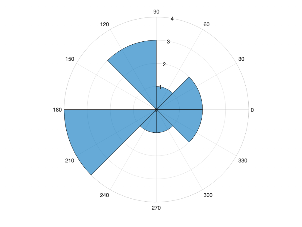
Figure 8.10: Polar histogram
After the histogram grid is constructed, the polar histogram is constructed in order to determine the direction that the robot should travel. Since the polar histogram describes the obstacle density of a given sector around the robot, the path can be adjusted in order to avoid regions that have lots of obstacles and may be unpassable. In particular, the robot should adjust its direction to attempt to continue toward its goal and select a sector that has a low obstacle density which will allow for smooth and safe travel. A 1D polar histogram has an angular resolution of [latex]\alpha[/latex] for a given number of sectors [latex]n[/latex]. This can be represented by [latex]\alpha = 360^{\circ}/n[/latex] and a breakdown for [latex]n = 8[/latex] in Figure 8.10. The obstacle density for a given sector of the polar histogram is calculated by Equation (8.11).
8.2.6 Polar Histogram Example Implementation
The following video shows a demonstration of a mobile robot using a lidar sensor to read its surroundings. The data from the lidar sensor is transformed and the strategies discussed in the vector filed histogram section are utilized to update the direction the robot is traveling. We do not implement a goal for this example but instead let the robot randomly search the space. The polar plot gives a representation of the density of objects in a given direction. In particular, we subdivide by the circle 18 times such that each region covers 20° degrees. We instruct the robot to rotate when the object density surpasses a given threshold in the -40º to 40º range, which is in front of the robot. We utilize the Coppeliasim simulator, the Remote Python API, and Python libraries such as Matplotlib and Numpy.
8.4 Summary
The ability for a robot to navigate an unstructured environment is one that is challenging, and many solutions have been developed through years of research. With the growing use of robotics in these types of environments, it is essential to continue developing and building upon these techniques to create more robust navigation systems. The introduction to navigation techniques in the chapter, such as fuzzy logic and SLAM algorithms, just scratches the surface of the complex navigation systems employed in robotics when techniques are combined. Additionally, the sensors presented in this chapter, such as LIDAR and Sonar, only give a small set of the total sensors available for the field of robotics. However, by understanding these baseline concepts, the reader now has a foothold in exploring the field of mobile robot navigation and assisting in developing systems to explore and save lives in the future.
Practice Questions
- Question 1: Compare the advantages and disadvantages of utilizing a lidar sensor vs an odometry sensor to navigate an unknown environment.
Answer: This answer does not include all advantages and disadvantages but covers a few key points. Lidar provides a very accurate and quick measurement of the surrounding of the environment which can be used in order to determine the position of obstacles around the environment. Lidar does however produce a large amount of data which may require a larger computational unit in order to perform processing. Additionally, many techniques that consume lidar data for control or planning are complex computational operations that also require more powerful computational resources. Odometry is a simpler sensor that allows a robot to know how far it has traveled based on determining the angle that the wheel has rotated and the radius of the wheel. This method is computationally simple and provides concise information about the position of the robot. However, odometry sensors are often subject to more error in their measurement when compared to lidar sensors.
- Question 2: What are the differences between local motion planning and global motion planning methods?
Answer: global path planning provides the overall goal position of the robot with a path that is constructed using a coarse granularity of knowledge about the region. Local motion planning updates the global path as it traverses an unknown environment based on the fine granularity knowledge it collects. By combining both methods a robot has a much better chance to traverse an area without getting stuck.
- Question 3: Given the polar histogram sector in the figure below containing the weights to detected obstacles in the grid cells calculate the obstacle density of for the sector. The constants are defined as follows [latex]a = 1/10[/latex], [latex]b = 1/100[/latex], assume [latex]c_{ij} = 10[/latex] for all grid squares.
![]()
Answer: 61
- Question 4: Determine whether the following node would be activated given a set of weights [latex][0.1,0.4,0.3,0.2][/latex], a set of inputs [latex][0.3334,0.1342,0.5234,0.8762][/latex], a bias value of [latex]0.2[/latex], and a threshold of [latex]0.5[/latex]. The activation function is given by the equation [latex]S(x) = \frac{1}{1+e^{-x}}[/latex].
Answer: Calculated value 0.65005 and the threshold is surpassed.
- Question 5: Determine the distance measured by a lidar sensor given a time of [latex]0.605 * 10^{-6} s[/latex] and speed of light [latex]299792458 m/s[/latex],
Answer: 181.37 m
References
[1] What Is SLAM (Simultaneous Localization and Mapping) – MATLAB & Simulink. (n.d.). Retrieved November 5, 2021, from https://www.mathworks.com/discovery/slam.html
[2] Sasiadek, J. Z., & Hartana, P. (2000). Sensor data fusion using Kalman filter. Proceedings of the Third International Conference on Information Fusion, 2, WED5/19-WED5/25 vol.2. https://doi.org/10.1109/IFIC.2000.859866
[3] Capi, G., Kaneko, S., & Hua, B. (2015). Neural Network based Guide Robot Navigation: An Evolutionary Approach. Procedia Computer Science, 76, 74–79. https://doi.org/10.1016/j.procs.2015.12.279
[4] Kim, Y., & Bang, H. (2018). Introduction to Kalman Filter and Its Applications. In Introduction and Implementations of the Kalman Filter. IntechOpen. https://doi.org/10.5772/intechopen.80600
[5] Faisal, M., Hedjar, R., Al Sulaiman, M., & Al-Mutib, K. (2013). Fuzzy Logic Navigation and Obstacle Avoidance by a Mobile Robot in an Unknown Dynamic Environment. International Journal of Advanced Robotic Systems, 10(1), 37. https://doi.org/10.5772/54427
[6] Yim, W. J., & Park, J. B. (2014). Analysis of mobile robot navigation using vector field histogram according to the number of sectors, the robot speed and the width of the path. 2014 14th International Conference on Control, Automation and Systems (ICCAS 2014), 1037–1040. https://doi.org/10.1109/ICCAS.2014.6987943
[7] Zhao, T., & Wang, Y. (2012). A neural-network based autonomous navigation system using mobile robots. 2012 12th International Conference on Control Automation Robotics Vision (ICARCV), 1101–1106. https://doi.org/10.1109/ICARCV.2012.6485311
[8] Holt, C, & Wang, Y. (2021). Ch8_MobileRobotNavigationSystem. Github, https://github.com/ClemsonFall2021ME8930IntroRobotics-HRI/Ch8_MobileRobotNavigationSystem
