
10 Impedance Control
Yehua Zhong
Chapter 10 Impedance Control
10.1 Task Space Dynamics
9.1.1 Dynamic Model
9.1.2 Examples
10.2 Impedance Control
9.2.1 Task Space Controller Design
9.2.2 Admittance Controller Design
10.3 Application
9.3.1 Human Arm Behavior
9.3.2 Choice of Impedance Control
10.4 Summary
Practice Questions
Simulation and Animation
References
Introduction
Impedance control is a prominent method in robotic dynamics control relating to force. It is based on the motion dynamics in joint space and transfer the dynamics to the task space to complete the control command. It is used in human-robot interaction applications often that the manipulator of the robot interacts with environment. Examples of applications include humans interacting with robots. In this chapter, we will explain how what the impedance control is and how we derive the model dynamics from joint space to task space as well as the choice of the impedance control law.
10.1 Task Space Dynamics
This section introduces the derivation of the impedance control in task space and how to use understand the dynamics between the virtual model and the external force from the environment. when it comes to robotic applications, one of the most common one is the impedance control nowadays, and according to the physical respond from the robot, impedance control can greatly help robots to interact with human to accomplish lots of tasks. To understand how the virtual model works in task space greatly help us to get into the impedance controller design logic.
10.1.1 Dynamic Model
Impedance control addresses a dynamic behavior between the robot end-effector and environment. To understand the change of dynamics of the robot end effector as well as how reaction forces are generated in association with environment, let’s start with the mass-spring-damper equations and derive the dynamics model to a generalized impedance dynamic. The following Lagrangian formular (9.1) describes an uncontrolled robot end-effector’s motion in joint space:
[latex]\tau = M(q)\ddot{q}+C(q,\dot{q})+g(q)+h(q,\dot{q}))+\tau_{ext}[/latex] (10.1.1)
[latex]q[/latex], [latex]\dot{q}[/latex], [latex]\ddot{q}[/latex] and in the equation (10.1) describe each joint’s angular position, angular velocity, and angular acceleration in joint space. represents the inertia matrix, represents the Coriolis and centrifugal torque, represents the gravitational torque, includes other possible existent torques including friction, stiffness of the joints, etc. [latex]\tau_{ext}[/latex] represents all other external forces from the environment. [latex]\tau[/latex] is the force input that we want to send to the robot.
Next, we can apply a common control law which is used as an example for demonstration.
[latex]\tau = K(q_d-q)+D(q_d-q)+g(q)+\hat{M}(q)\ddot{q}+\hat{g}+\hat{h}(q,\dot{q})[/latex] (10.1.2)
[latex]K[/latex] and [latex]D[/latex] are the control parameters as stiffness and damping coefficients. [latex]\hat{M},\ \hat{c},\ \ \hat{g},\ \ \hat{h}[/latex] are the dynamic parameters that we have in the robot from equation (10.1). Assume [latex]q_d[/latex] is the desired angular position that we want, and is the actual joint angular position. If we insert the equation (10.1) to equation (10.2), a controlled robot system is described as following equation:
[latex]K(q_d-q)+D(\dot{q}_d-\dot{q})+M(q)(\ddot{q}_d-\ddot{q}) = \tau_{ext}[/latex] (10.1.3)
[latex]\tau_{ext}[/latex] is applied by the environment, where describe the stiffness and damping of the closed loop system. Based on the changing of our external forces we will have the corresponding controlled robot behavior. For example, if we want to obtain the joint acceleration ([latex]\ddot{q}[/latex]) or velocity ([latex]\dot{q}[/latex]), we can utilize the equation above by giving an input force ([latex]\tau_{ext}[/latex]), then our designed stiffness ([latex]K[/latex]) and damping ( would help us get the corresponding velocity and acceleration according to specific tasks, we can then input the velocity or acceleration to the robot to finish the control command. To further understand, the values of the stiffness ([latex]K[/latex]) and damping ([latex]D[/latex]) are the key to decide the motion dynamics of the end-effector, for example, if the stiffness ( is a relatively big number, the robot end-effector is expected to have a stiffer motion.
When it comes to task space, we can replace the joints’ angular velocity and acceleration ([latex](\ddot{q},\dot{q}[/latex]) with generalized coordinates ([latex]\ddot{x},\dot{x}[/latex]) to the Lagragian formular in joint space, and we get the following equation:
[latex]F = \mathrm(q)\ddot{x}+\mu(x,\dot{x})+\gamma(q)+\eta(q,\dot{q})+F_{ext}[/latex] (10.1.4)
[latex]\mathrm{\Lambda}\left(q\right)\ddot{x}+\mu\left(x,\dot{x}\right)[/latex] describes the dynamics model of the robot in task space where can be solved for using the joint angular position and velocity that describe the generalized gravitation, and further terms. is the input force from the environment in task space.
Similarly, to the joint space control law, the following equation describes the control law in task space.
[latex]F = K_x(x_d-x)+D_x(\dot{x}_d-\dot{x})+\hat{\mathrm{\Lambda}}(q)\ddot{x}_d+\hat{\mu}(q,\dot{q})+\hat{\gamma}(q)+\hat{\eta}(q,\dot{q})[/latex] (10.1.5)
[latex]K_x[/latex] and [latex]D_x[/latex] are the task space stiffness and damping matrices, [latex]\hat{\mathrm{\Lambda}},\ \hat{\mu},\hat{\gamma},\hat{\eta}[/latex] are the internal model of the robot mechanism. Meanwhile, we should pay attention to the trade-off between the position accuracy and the contact forces from environment.

As the [latex]Figure 10.1.1[/latex] above shows that a 4-link robot with an external force from the environment, we could envision all the links and joints of the robot would perform in different ways according to the changes of the external force. Apparently, a good, designed controller should take sensors and actuators into considerations, because multiple linkages and actuators would have more degrees of freedom to influence the controller to balance the dynamic relationship between the environment and the robot. How to determine the proper stiffness coefficient and damping coefficient could be the limitations of the impedance control application.
10.1.2 Examples
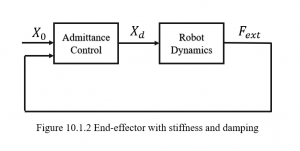
The robot is an impedance control, it has damping and stiffness to smooth the motion shown in [latex]Figure 10.1.2[/latex], whenever we have a force applied from the environment, the stiffness and damping of the robot would adjust the motion of the end-effector based on the dynamic model. During the robot-human interaction, impedance control plays an important role in robots’ manner to keep the interaction safe. For example, a robot is assisting human lifting heavy weight objects, if we are using the position control to manipulate the robot to achieve the task, which means the robot will move to the assigned position in task space without taking any other factors into consideration. If the weight is over the maximum payload of the robot, it not only might cause the robot fail but also lead to injury of human. If we use impedance control on the robot, based on the dynamic model, we have damping and stiffness to adjust the motion, the robot could smooth the motion and return to certain positions without oscillations.
10.2 Impedance Control
Impedance controller gives a spring-damper system in dynamic relationship between the human and robot, this section provides an idea about how do we use the virtual model to design a proper impedance controller. By using the impedance or admittance controller in Cartesian space, which gives us a clear picture of how the manipulator would behave when it responses to external force as well as internal stiffness and damping parameters.
10.2.1 Task Space Controller Design
Based on the dynamic models from 10.1.1, an impedance control law is to modulate the impedance parameters to be effective to the robot end-effector. The following dynamics model tells us another good impedance control law in task space.
[latex]F = J\hat{}T({\theta})(\widehat{\Lambda} )({\theta})\ddot{x}+\tilde{\eta}(\theta,\dot{x})-(M\ddot{x}+B\dot{x}+Kx))[/latex] (10.2.1)
The dynamics compensation as well as the change of the external force applied from the environment provide a good feedback system to allow the end effector of the robot to achieve more closely to the desired position. The arm dynamics compensation in this equation transferred from the joint space to task space.
For human factor in such interaction, we take human as a admittance in the system, to better understand the concept of the admittance control, let’s start with the mass-spring-damper system.
[latex]m\ddot{x}+b\dot{x}+kx = f[/latex] (10.2.2)
Where is the position, is the damping coefficient, is the stiffness coefficient, and is the force applied by the environment (could be human or force input from the environment). Based on the equation (10.7), we notice that different force input influences the position, velocity, and acceleration of the robot. Furthermore, if we transfer the function above into a frequency domain by using the Laplace transformation, we have
[latex](ms^2+bs+k)X(s) = F(s)[/latex] (10.2.3)
The impedance is defined as [latex]Z\left(s\right)=\ \frac{F(s)}{X(s)}[/latex] . In mechanical dynamics, the impedance is the amount of resistance in a motion subjected to a force, the ratio of the input to output in transfer function tells us how much the impedance exists in the motion, if the impedance is a very large number compared to the input force, [latex]F\left(s\right)=Z\left(s\right)X(s)[/latex] tells us that the position, velocity, or acceleration would barely change. The inverse of the impedance is the admittance, [latex]Y\left(s\right)=\ Z^{-1}\left(s\right)=\ \frac{X(s)}{F(s)}[/latex] , that is the ratio of output to input tells us that if the admittance is a very large number, a small force input could cause the position, velocity or acceleration have a big change. We could simply introduce that the impedance control is described as robot, and admittance control represents the environment.
10.2.2 Admittance Controller Design
As one of the common methods to interact with robot, admittance control provides a dynamic balance in the interaction between human and robot. Normally, a force sensor is installed on the end effector of the robot and by sensing the external force from the environment, a good admittance controller is able to provide the dynamic model for the desired movement of the robot with corresponding velocity, acceleration.
The simplified block diagram tells us how the admittance control works within the interaction between human and robot. By receiving the initial condition (position, velocity, acceleration), the admittance controller sends out a correspondingly desired position, velocity, acceleration to the robot. More specifically, we can use the equations below to understand how the block diagram works in a mathematical way.
[latex]M_a\ddot{x}_d = -D(\dot{x}_d-x)-K(x_d-x)+F_{ext}[/latex] (10.2.4)
The [latex]Equation (10.2.4)[/latex] is different from the Equation (10.5) because here we don’t have a specific robot mechanism. Therefore, if we want to a most accurate acceleration, we not only need to design a proper damping and stiffness coefficient but also obtain the specific mechanism data of the robot.
10.3 Application
Daily applications are realistic and more serious than virtual spring-damper modal, there are still lots of limitations when it comes to the application of the impedance control but bringing robots into unstructured environments has its great advantages that has been proved in industrial, hospital, and many other fields. This section would explain how the interaction between human and robot with some innovative models as well as controllers that came out just a couple of years ago.
10.3.1 Human Arm Behavior
The increasing demand for robotic assistance in some industry has made impedance control more and more popular in recent years since it provides a reactive and safe environment while the robot is assisting the work. Variable impedance control (VIC) was first presented by Ikeura and Inooka for this cooperative system (1995) in 1995. Let’s assume two humans are performing a heavy task job (lifting a heavy object), it is easy and quick for the human to adjust the force to balance the lift, in addition, moving direction’s intention is easy to be detected from human’s sense. However, when it comes to human robot cooperation in assisting such heavy task, a small force change could lead to huge impact (admittance control) on the robot’s performance. In 2019, Murator (2019) et al. proposed a multimodal interaction framework that help to solve this uncertainty by using the equation:
[latex]K_t = K_0+\alpha e^2_t[/latex] (10.3.1)
Where the Kt is the joint stiffness for each joint, and k0 is a small stiffness used to smooth the interaction, and et is the error (trajectory error), alpha is a positive gain. Adding more stiffness to the system let the end effector reach the desired position more accurately.
10.3.2 Choice of Impedance Control
There are lots of well-designed controllers in industrial robots nowadays when they are manufactured, many applications in different fields would have all kinds of distinct controllers based on specific requirements, controllers are like brains to human that they can control the behavior of robots. For example, KASKAWA’s Motoman XRC robot controller has been on the market for decades that they are able to control up to 6-axis robot and are compatible with many robots nowadays.
According to the models introduced in this chapter, it is not hard to realize that the stability of impedance control is the key during the human robot interaction. One of the earliest stability analyses of VIC was for a force tracking impedance controller (Lee and Buss, 2008). The controller model was using the previous dynamics error to adjust the robotic stiffness that led to a second order linear time varying system. The unstructured environment brings a huge challenge to the stability of the impedance control that different model can be applied due to specific tasks. Classical robotics, mostly characterized by high gain negative error feedback control, is not suitable for tasks that involve interaction with the environment (possibly humans) because of possible high impact forces. The use of impedance control provides a feasible solution to overcome position uncertainties and subsequently avoid large impact forces, since robots are controlled to modulate their motion or compliance according to force perceptions (Dakka, 2019).
10.4 Summary
The growth in robot applications and technologies already changed the world’s view to the robots. In the past, robot would only do single task with repetitive mechanical motion. Now the mechanical motion becomes more intelligent due to robot controller which allows the robot to have a “brain” that utilize the designed virtual model to accomplish specific tasks. When it comes to more advanced robot controller like impedance control, it is feasible that this kind of control law provides a solution to the uncertainty and unsafety. Since The uncertainty and unsafety are dynamic, it requires the controller to be very specific for its parameters design based on different kinds of robot. It would be more and more diverse in different kinds of robot and robot controllers.
Practice Questions
References
Abu-Dakka Fares J., S. M. (2020). Variable Impedance Control and Learning—A Review. Frontiers in robotics and AI, 177.
Abu-Dakka, F. J. (2020). Variable Impedance Control and Learning-A Review. Frontiers in robotics and AI, vol. 7.
AUTHOR=Abu-Dakka Fares J., S. M. (2020). Variable Impedance Control and Learning—A Review . Frontiers in Robotics and AI , 177.
Ikeura R., I. H. (1995). Variable impedance control of a robot for cooperation with a human. IEEE International Conference on Robotics and Automation, 3097-3102.
Muratore L., L. A. (2019). A self-modulated impedance multimodal interaction framework for human-robot collaboration. IEEE International Conference on Robotics and Automation (ICRA) (pp. 4998–5004). Montreal: ICRA.
Pitakwatchara, P. (2014). Task Space Impedance Control of the Manipulator Driven Through the Multistage Nonlinear Flexible Transmission. Control, ASME.
