
2 Forward Kinematics
Ashley Stevens
Forward Kinematics Outline
2.1 Rotation & Homogeneous Matrices
2.2 Simple Trigonometry Method
2.2.1 Representing Position
2.2.2 Representing Rotation
2.2.2.1 Planar Rotation
2.2.2.2 Rotation Rules
2.2.2.1 Three-Dimensional Rotation
2.2.3 Rigid Motions
2.2.4 Homogeneous Transformation
Example – Homogeneous Transformation
2.3 Kinematic Chains
2.4 Trigonometry Method
Example – Two-Link Planar Manipulator (Trigonometry Method)
2.5 Denavit-Hartenberg Parameter
Example – Two-Link Planar Manipulator (DH Convention)
2.6 Screw Theory
2.6.1 Twists
Example – Twists
2.6.2 Screw Theory Procedure
Example – Screw Theory in {s} frame
2.7 Summary
2.8 Properties to Know for the Practice Questions
Practice Questions
Simulation and Animation
References
Introduction
Kinematics overall describes the manipulator’s motion. Forward kinematics is used to calculate the position and orientation of the end effector when given a kinematic chain with multiple degrees of freedom.
To start, we will see a light overview of the robot components before launching into the basics of forward kinematics: rotation matrices, rigid motion, and homogeneous transformation. From there we will discuss three different methods on how to solve a forward kinematics problem: trigonometry, Denavit-Hartenberg convention and screw theory.
2.1 Robot Components
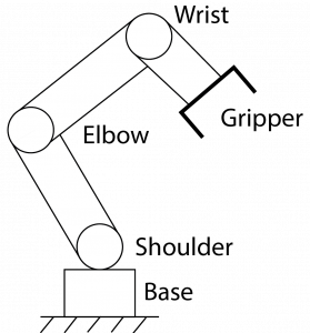
An articulated robot is composed of the base, shoulder, elbow, spherical wrist, and gripper. The base is an anchor point that supports the unit. The shoulder and elbow are jointed allowing the robot to move. The wrist is attached to the jointed arm and at the end of it is the gripper.
Each joint, like the elbow, can be classified as a revolute (R) joint or a prismatic (P) joint. These actuators are movable parts and cause relative motion between the two links it connects.
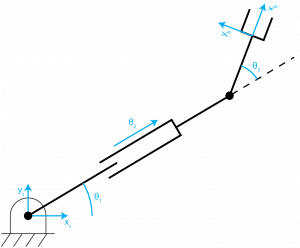
A revolute joint, as shown in Figure 2.2, has 1 degree of freedom (DoF). The axis of rotation of a revolute joint becomes the zi axis. It also has a joint variable, θi, representing the relative displacement between link i-1 and link i. For this chapter, the joint variable will always be represented in units of degrees.

A prismatic joint, as shown in Figure 3, has 1 DoF. The axis of translation becomes the zi axis as illustrated in the figure. The relative displacement of this joint is represented by di and is in units of meters.

There are other types of joints such as a ball and socket (2 DoF) or a spherical wrist (3 DoF). However, for simplicity, only a revolute and/or a prismatic joint type (1 DoF) will be used during this chapter.
Another important component of the robot is the rigid body. A rigid body is the link that connects the shoulder joint to the elbow joint is a link.
In addition to rigid bodies, the robot contains kinematic chains. A kinematic chain is the grouping of links and joints that produce the desired motion. A human arm or a human leg are two examples of kinematic chains.
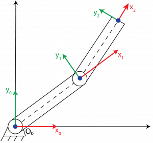
In Figure 2.1, the gripper is the end-effector of that kinematic chain. The end effector interacts with the environment around the robot. The type of end effector can change based on the robot’s usage: gripper, welding gun, magnet, force-torque sensors, tool changers.
2.2 Rigid Motion and Homogeneous Matrices
This section provides an overview on how to represent the position of a point with an analytical approach. It also shows how to represent planar and three-dimensional rotations and the rules of rotation matrices. In addition, rigid motions and homogeneous transformations will be covered.
2.2.1 Representing Position
To represent our position, we will be setting up a coordinate frame and showing how to represent a position with respect to different frames. This is due to robotics typically using the analytic reasoning due to tasks often being defined in Cartesian coordinates. Figure 2.4 shows two coordinate frames that differ by 45°.

The point can be defined with respect to frame {0},
[latex]p^0=\begin{bmatrix} 5\\ 6 \end{bmatrix}[/latex]
or with respect to frame {1},
[latex]p^1=\begin{bmatrix} -2.8\\ 4.2 \end{bmatrix}[/latex]
p is a geometric entity that is a specific location in space while p0 and p1 represent the point’s location with respect to each coordinate frame. The p0 and p1 are coordinate vectors. The origin, also a point in space, is also assigned a coordinate frame. The following notations both represent the same origin point. The first notation represents the origin in frame {1} with respect to frame {0}. The second notation represents the origin in frame {0} with respect to frame {1}.
[latex]o_1^0=\begin{bmatrix} 10\\ 5 \end{bmatrix}[/latex], [latex]0_0^1=\begin{bmatrix} -10.6\\ 3.5 \end{bmatrix}[/latex]
The subscript can be omitted if there is only a single coordinate frame or when the reference frame is obvious. However, this is not suggested as it is poor technique.
2.2.2 Representing Rotation
Rotations can be represented in planar (two-dimensional) and three-dimensional terms. Along with this, there are some rules that should be kept in mind when working with rotation matrices that will be touched upon at the end.
2.2.2.1 Two-Dimensional Rotations
The rotation matrix, [latex]R_1^0[/latex], is created by projecting the axes of frame {1} onto the coordinate axes of frame {0} as shown with the following.
[latex]R_1^0=\begin{bmatrix} x_1 \cdot x_0 & y_1 \cdot x_0\\ x_1 \cdot y_0 & y_1 \cdot y_0 \end{bmatrix}[/latex] (2.1)
The rotation matrix has column vectors that are comprised of the unit vectors’ coordinates along the axes of frame {1} with respect to frame {0}.
Example – Planar Rotation
Below is an illustration of a planar rotation with frames {0} and {1}.
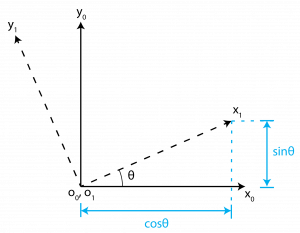
For this planar rotation, the rotation matrix can be calculated as,
[latex]R_1^0 = \begin{bmatrix} x_1^0 y_1^0 \end{bmatrix}[/latex] (2.2)
[latex]R_1^0 = \begin{bmatrix} cos \theta & -sin\theta\\ sin\theta & cos\theta \end{bmatrix}[/latex] (2.3)
This rotation matrix, [latex]R_1^0[/latex], is representing the orientation of frame {1} with respect to frame {0}.
2.2.2.2 Rules of Rotation Matrices
[latex]R_1^0[/latex] column vectors are mutually orthogonal and are of unit length. Thus, the matrix is orthogonal and the det([latex]R_1^0[/latex]) = ±1. Since we use the right-hand rule to set up the coordinate frame, det([latex]R_1^0[/latex]) = +1. Due to this, we can refer to such n x n matrices as Special Orthogonal group of order n (SO(n)).
For any the following properties are true,
- [latex]R^T = R^{-1} ∈ SO(n)[/latex]
- The columns (and rows) of R are mutually orthogonal
- Each column (and row) of R is a unit vector
- det(R)=1
We now have the rotation matrix of frame {1} with respect to frame {0}. However, we also want the reverse: the rotation matrix of frame {0} with respect to frame {1}; then the following equation can be used.
[latex]R_0^1 = (R_1^0)^T[/latex] (2.4)
Consider having a fixed frame of {0} and a current frame of {1}, which results in a rotation matrix [latex]R_1^0[/latex]. Then a third frame is brought in {n} and related to the current frame {1}. With this there is a resulting rotational matrix of [latex]R_n^1[/latex]. To obtain [latex]R_n^0[/latex], post-multiplication can be used. Post-multiplication simply means that the new term, [latex]R_n^0[/latex], is multiplied at the end of the current sequence.
[latex]R_n^0 = R_1^0 R_n^1[/latex] (2.5)
This shows the transformation of frame {0} with respect to frame {n}.
One of the most important rules involves the multiplying of matrices. The rotation matrix should be pre-multiplied when the rotation is about a fixed/world frame. The rotation matrix should be post-multiplied when the rotation is about the current frame.
2.2.2.3 Three-Dimensional Rotations
The same process used in the two-dimensional rotations is used to have a resulting rotational matrix of three dimensions where the three axes of frame {1} is projected onto frame {0}.
[latex]R_1^0 = \begin{bmatrix} x_1 \cdot x_0 & y_1 \cdot x_0 & z_1 \cdot x_0\\ x_1 \cdot y_0 & y_1 \cdot y_0 & z_1 \cdot y_0 \\ x_1 \cdot z_0 & y_1 \cdot z_0 & z_1 \cdot z_0 \end{bmatrix}[/latex] (2.6)
This belongs to group as it is orthonormal with a determinant equal to 1.
Example – Basic Rotation Matrix about z0-axis
The frame {1} is rotated through an angle θ about the z0-axis. Find the resulting transformation matrix, [latex]R_1^0[/latex].
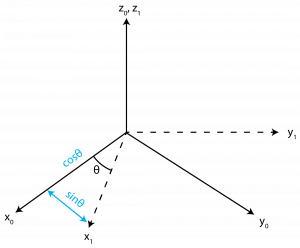
From the above figure, the following is determined
[latex]x_1 \cdot x_0 = cos \theta[/latex], [latex]y_1 \cdot x_0 = -sin \theta[/latex]
[latex]x_1 \cdot y_0 = sin \theta[/latex], [latex]y_1 \cdot y_0 = cos \theta[/latex]
[latex]z_0 \cdot z_1 = 1[/latex]
and the remaining dot products result in zero. This forms the following rotation matrix
[latex]R_1^0 = R_{z,\theta} = \begin{bmatrix} cos \theta & -sin \theta & 0\\ sin \theta & cos \theta & 0 \\ 0 & 0 & 1\end{bmatrix}[/latex] (2.7)
As this matrix can be applied to any rotation about a z-axis, the notation of [latex]R_{z,θ}[/latex] is interchangeable with [latex]R_1^0[/latex].
This same process is used to calculate rotations about the x– and y– axes.
[latex]R_{x,\theta} = \begin{bmatrix} 1 & 0 & 0\\ 0 & cos \theta & -sin \theta \\ 0 & sin \theta & cos \theta\end{bmatrix}[/latex] (2.8)
[latex]R_{y,\theta} = \begin{bmatrix} cos \theta & 0 & sin \theta\\ 0 & 1 & 0 \\ -sin \theta & 0 & cos \theta\end{bmatrix}[/latex] (2.9)
Example – Multiplying Rotational Matrices
Find the rotation matrix after the following rotations occur,
- Rotate by θ about the current x-axis
- Rotate by ф about the current z-axis
- Rotate by α about the fixed z-axis
- Rotate by β about the current y-axis
- Rotate by γ about the fixed x-axis
Start with the rotation number 1 then pre- or post-multiply by each next rotation.
[latex]R=R_{x,\gamma}R_{z,\alpha}R_{x,\theta}R_{z,\phi}R_{y,\beta}[/latex]
Note: moving forward cosine will be abbreviated to c and sine will be abbreviated to s with the subscript indicating the angle used for the respective trigonometric function. If there are two subscripts to a single trigonometry function, those angles are added together before being used in said function.
2.3 Rigid Motion
A pure translation coupled with a pure rotation is considered a rigid motion. We will be using the rotation matrices as defined previously along with d, a vector from frame {0} origin to frame {1} origin. Suppose in frame {1}, we know of a point p rigidly attached with local coordinates making it p1. To then express this point with respect to frame {0}, the following is used
[latex]p^0=R_1^0p^1+d^0[/latex] (2.10)
To illustrate, consider wanting to know the location of the blue dot, p0, in the following coordinate frame, frame {0}.
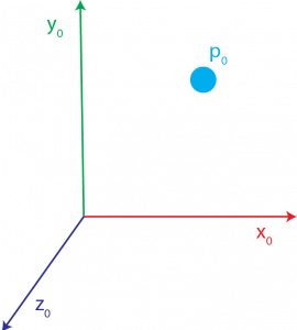
However, you only have the location of the point, p1, in frame {1} with the known rotation matrix, [latex]R_1^0[/latex], and the distance between the origins, d0.
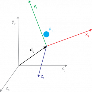
This is when you would use Equation (2.10) to find the location of the blue dot in frame {0}.
To advance this concept, consider having three frames: frame {0}, {1}, and {2}. Where d1 is a vector from the origin of frame {0} to the origin of frame {1} and d2 is the vector from the origin of frame {1} to the origin of frame {2}. The point p is represented as p2 in frame {2}. We wish to compute it relative to frame {0} with the following process.
[latex]p^1=R_2^1p^2+d_2^1[/latex] (2.11)
[latex]p^0=R_1^0+p^1+d_1^0[/latex] (2.12)
Equation (2.12) is rearranged and substituted into Equation (2.11) to create
[latex]p^0=R_1^0R_2^1p^2+R_1^0d_2^1+d_1^0[/latex] (2.13)
Due to the following two relationships,
[latex]R_2^0=R_1^0R_2^1[/latex] (2.14)
[latex]d_2^0=d_1^0+R_1^0d_2^1[/latex] (2.15)
Equation (2.13) can be re-written as the following,
[latex]p^0=R_2^0p^2+d_2^0[/latex] (2.16)
2.2.4 Homogeneous Transformation
Putting the rigid motion into a matrix representation is to create a homogeneous transformation. It combines the rotation and translation previously discussed into a single matrix multiplication. The homogeneous matrix (H) is used for coordinate transformations,
[latex]H=\begin{bmatrix} R & d\\ 0 & 1\end{bmatrix}, R\in SO(3), d \in \mathbb{R}^3[/latex](2.17)
Similar to the rotation matrix rules, the inverse transformation is given by
[latex]H^{-1}=\begin{bmatrix} R^T & -R^Td \\ 0 & 1\end{bmatrix}[/latex] (2.18)
The following are a set of basic homogeneous transformations. Equation (2.19) shows the translation in the x-axis direction by a unit(s) as well as a rotation about the x-axis by α degree(s).
[latex]Trans_{x,a} = \begin{bmatrix} 1 & 0 & 0 & a\\ 0 & 1 & 0 & 0 \\ 0 & 0 & 1 & 0 \\ 0 & 0 & 0 & 1 \end{bmatrix}[/latex], [latex]Rot_{x,\alpha} = \begin{bmatrix} 1 & 0 & 0 & 0\\ 0 & c_\alpha & -s_\alpha & 0 \\ 0 & s_\alpha & c_\alpha & 0 \\ 0 & 0 & 0 &1\end{bmatrix}[/latex] (2.19)
Equation (2.20) shows the translation in the y-axis direction by b unit(s) as well as a rotation about the x-axis by β degree(s).
[latex]Trans_{y,b} = \begin{bmatrix} 1 & 0 & 0 & 0\\ 0 & 1 & 0 & b \\ 0 & 0 & 1 & 0 \\ 0 & 0 & 0 & 1 \end{bmatrix}[/latex], [latex]Rot_{y,\beta} = \begin{bmatrix}c_\beta & 0 & s_\beta & 0\\ 0 & 1 & 0 & 0 \\ -s_\beta & 0 & c_\beta & 0 \\ 0 & 0 & 0 &1\end{bmatrix}[/latex] (2.20)
Equation (2.21) shows the translation in the x-axis direction by c unit(s) as well as a rotation about the x-axis by γ degree(s).
[latex]Trans_{z,c} = \begin{bmatrix} 1 & 0 & 0 & 0\\ 0 & 1 & 0 & 0 \\ 0 & 0 & 1 & c \\ 0 & 0 & 0 & 1 \end{bmatrix}[/latex], [latex]Rot_{x,\alpha} = \begin{bmatrix} c_\gamma & -s_\gamma & 0 & 0\\ s_\gamma & c_\gamma & 0 & 0 \\ 0 & 0 & 1 & 0 \\ 0 & 0 & 0 &1\end{bmatrix}[/latex] (2.21)
It is important to note the previously stated rotation matrix rules also apply to homogeneous matrices.
Example – Homogeneous Transformation
Find a homogeneous transformation matrix that represents a rotation of angle α about the current x-axis, a translation of b along the current x-axis, a translation of d along the current z-axis, and a rotation of angle θ about the current z-axis.
[latex]H=Rot_{x,\alpha}Trans_{x,b}Rot_{z,\theta}=\begin{bmatrix} c_\theta & -s_\theta & 0 & b\\ c_\alpha s_\theta & c_\alpha c_\theta & -s_\alpha & -ds_alpha \\ s_alpha s_\theta & s_alpha c_\theta & c_\alpha & dc_\alpha \\ 0 & 0 & 0 & 1\end{bmatrix}[/latex]
2.3 Kinematic Chains
As previously touched on, a robot is comprised with links that are connected by joints (R or P) that make up a kinematic chain.
For a robot with n links there will be n+1 links. To label a robot, the joints are labelled 1 to n while the links are labelled 0 to n with the base being the start. The first link, the base, is always fixed and does not move when any joints are actuated.
In addition to labeling the joints a joint variable, qi, is included.
[latex]q_i=\begin{Bmatrix} \theta_i & \textrm{if joint $i$ is revolute}\\ d_i & \textrm{if joint $i$ is prismatic}\end{Bmatrix}[/latex] (2.22)
For a visualization of Equation (2.22), refer back to Figure 2.2 for a revolute joint and Figure 2.3 for a prismatic joint.
The previously calculated homogeneous transformation matrix that expressed position and orientation of frame {j} with respect to {i} now takes on a new name: a transformation matrix, [latex]T_j^i[/latex]
[latex]T_j^i=\begin{Bmatrix} A_{i+1}A_{i+2}...A_{j-1}A_{j-2} & \textrm{if $ii$}\end{Bmatrix}[/latex] (2.23)
where the homogeneous transformation Ai is the following. It uses [latex]o_i^{i-1}[/latex], a three-vector that indicates the end effector position and orientation with respect to the base frame.
[latex]A_i=\begin{bmatrix} R_i^{i-1} & o_i^{i-1}\\ 0 & 1 \end{bmatrix}[/latex] (2.24)
2.4 Trigonometry Method
For the trigonometric method, a robot is placed into a 2-D planar coordinate system. From here, the angles between each joint movement are found to be able to use the trigonometric functions to find the end effector location with respect to the base joint.
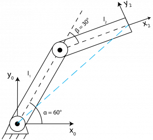
Example – Two-Link Planar Manipulator (Trigonometry Method)
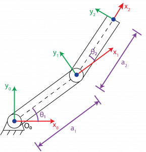
The first joint is mounted to the base, so it is fixed but still able to rotate. The first joint is rotated by 60° (α). The first and second joints are connected by link one with a length of l1. The second joint is rotated by 30° (β). The second joint is connected to the end effect via link two with a length of l2. Let l1 = l2 = 1. Find the coordinates of the end effector (x2, y2).
| [latex]x'=l_1cos\alpha[/latex] | [latex]y'=l_1sin\alpha[/latex] |
| [latex]x"=l_2cos(\alpha+\beta)[/latex] | [latex]y"=l_2sin(\alpha+\beta)[/latex] |
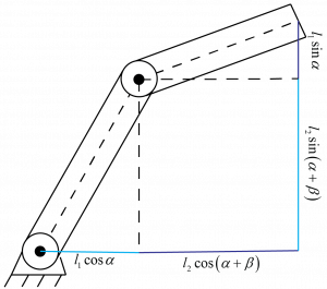
[latex]x=l_1cos\alpha + l_2cos(\alpha+\beta)[/latex]
[latex]x=\frac{1+\sqrt{3}}{2}[/latex]
[latex]y=l_1sin\alpha+l_2sin(\alpha+\beta)[/latex]
[latex]y=\frac{1+\sqrt{3}}{2}[/latex]
2.5 Denavit-Hartenberg Convention
The Denavit-Hartenberg (DH) convention is one of the most common for selecting reference frames for robots. With the DH convention, each Ai is represented as the following
[latex]A_i=Rot_{z,\theta}Trans_{z,d}Trans_{x,a}Rot_{x,\alpha}=\begin{bmatrix} c_\theta & -s_\theta c_\alpha & s_\theta s_\alpha & a c_\theta\\ s_\theta & c_\theta c_\alpha & -c\theta s_\alpha & as_\theta \\ 0 & s_\alpha & c_\alpha & d \\ 0 & 0 & 0 & 1\end{bmatrix}[/latex](2.25)
The following is a general procedure that can be used when implementing the DH Convention onto a forward kinematics problem.
Step 1: Draw out the robot
Illustrate the revolute and prismatic joints by setting the zi axis and the θi or di for the respective joint types.
Step 2: Assign the remaining axes
We’ve already assigned zi as the axes of rotation/translation for a revolute/prismatic joint, respectively. After that, the xi must be perpendicular to both the zi and zi-1 axis and it must intersect with zi-1. For the remaining axis, yi, it is determined with the right-hand rule. For the right-hand rule, the thumb is set as the z-axis, the index finger becomes the x-axis, and the y-axis is the middle finger.
Step 3: Assign the DH parameters (a, α, d, θ)
The link length, ai, is measured along xi and is the distance between zi-1 and zi.
The link twist, αi, is in a plane normal to xi and is the angle between zi-1 and zi.
The joint offset, di, is measured along zi-1 and is the distance from oi-1 to the intersection of xi and zi-1. If the joint i is revolute, then the joint offset is a constant value.
The joint angle, θi, is measured in a plane normal to zi-1 and is the angle between xi-1 and xi. If joint i is prismatic, then the joint angle is a constant value.
To have a more in-depth visualization of this see the following YouTube video by TekkotsuRbotics.
Step 4: Create a DH table
List all known values in a DH table. Any variable values should be denoted with an *.
You conclusion should summarize the main points of your chapter as a way of reminding the reader what they just learned.
| Links | ai | αi | di | θi |
| 1 | a1 | α1 | d1 | θ1 |
| … | … | … | … | … |
| i | ai | αi | di | θi |
Step 5: Calculate each Ai matrix
There will be an Ai matrix for the (i-1)th origin. The reference origin of 0 will never have an A matrix. Only origins after 0 will have an A matrix that can be calculated with Equation (2.25).
Step 6: Calculate the T matrix
Based upon the frames that are to be expressed, Equation (2.23) is used along with the previously calculated Ai matrix.
Example – Two-Link Planar Manipulator (DH Convention)
Consider the below two-link planar manipulator. Derive the forward kinematics equations using the DH-Convention.
As following our outlined steps, the axis for each joint needs to be established as shown in the following figure. All z-axes are normal to the page and are represented by each blue dot.
For step 3, the DH parameters are assigned.
With these established DH parameters, the DH table can be constructed for step 4. Keep in mind that frame 0 (link 0) is never included in the DH table.
| Link | ai | αi | di | θi |
| 1 | a1 | 0 | 0 | θ3* |
| 2 | a2 | 0 | 0 | θ2* |
From this table, the following A matrices can be determined using Equation (2.25) and completing step 5.
[latex]A_1=\begin{bmatrix} c_1 & -s_1 & 0 & a_1c_1\\ s_1 & c_1 & 0 & a_1s_1 \\ 0 & 0 & 1 & 0 \\ 0 & 0 & 0 & 1 \end{bmatrix}[/latex], [latex]A_2=\begin{bmatrix} c_2 & -s_2 & 0 & a_2c_2\\ s_2 & c_2 & 0 & a_2s_2 \\ 0 & 0 & 1 & 0 \\ 0 & 0 & 0 & 1 \end{bmatrix}[/latex]
With these A matrices, the following T matrices can be determined for step 6.
[latex]T_1^0 = A_1=\begin{bmatrix} c_1 & -s_1 & 0 & a_1c_1\\ s_1 & c_1 & 0 & a_1s_1 \\ 0 & 0 & 1 & 0 \\ 0 & 0 & 0 & 1 \end{bmatrix}[/latex]
[latex]T_2^0=A_1A_2=\begin{bmatrix} c_12 & -s_12 & 0 & a_1c_1+a_2c_12\\ s_12 & c_12 & 0 & a_1s_1+a_2s_12 \\ 0 & 0 & 1 & 0 \\ 0 & 0 & 0 & 1 \end{bmatrix}[/latex]
The x and y components of the origin in frame {2} are the first two entries in the last column of [latex]T_2^0[/latex]. Thus,
[latex]x=a_1c_1+a_2c_12[/latex]
[latex]y=a_1s_1+a_2s_12[/latex]
making up the end effector’s coordinators in the base frame. The first three entries in columns 1-3 make up the rotation part. This gives the orientation of frame {2} relative to the base frame of {0} as denoted by [latex]T_2^0[/latex].
2.6 Screw Theory
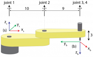
An alternative to the Denavit-Hartenberg convention is the screw theory. For the screw theory, only the coordinate system of the space {s} frame and the end effector coordinate system {b} frame need to be established. To calculate the transformation matrix T(θ), the product of exponential (PoE) is used and is based on the frame system chosen: {s} or {b} frame. The same multiplication rules with the rotation matrices are applied here, when the {s} frame is chosen, pre-multiplication is used. When the {b} frame is chosen, post-multiplication is used.
2.6.1 Twists
If a body has linear and angular velocity, then there is a corresponding screw axis.

The screw axis has a point q on the axis, a unit vector s in the direction of the axis, and the pitch h of the screw which is defined with Equation (2.26). The screw axis represents the direction the body is moving in. The [latex]\dot{θ}[/latex] is a scalar value representing the body’s rotation speed about the screw. This is illustrated in Figure 2.12. To start, we are going to look at finite pitch.
[latex]h=pitch=\frac{linear speed}{angular speed}[/latex] (2.26)
To represent the screw axis, a reference frame is chosen and the screw axis, S, is defined in the frame’s coordinates.
[latex]S=\begin{bmatrix} S_w\\ S_v \end{bmatrix}=\begin{bmatrix} angular velocity when \dot{\theta}=1\\ linear velocity of the origin when \dot{\theta}=1 \end{bmatrix}[/latex] (2.27)
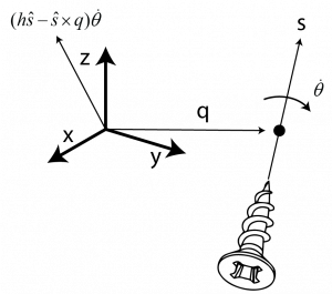
The linear velocity of the origin as shown in the above figure is split up into two terms times theta dot (a scalar rate of rotation). The first term, assuming there is a nonzero pitch, is the linear velocity due to the translation along the screw axis. The second term is the linear velocity due to the rotation about the screw axis. This creates the twist, V, a full representation of angular and linear velocity.
[latex]V=\begin{bmatrix} w\\ v \end{bmatrix}=S\dot{\theta}[/latex] (2.28)
Example – Simple Twist
In the following illustration, the screw axis is a zero-pitch screw with a pure rotation. The screw is pointing out of the screen, represented by the black dot. Imagine the dotted line rotates counterclockwise for the pure rotation. Find the angular and linear velocity.

| [latex]S_w=\begin{bmatrix} 0\\ 0 \\1 \end{bmatrix}[/latex] | [latex]S_v=\begin{bmatrix} 0\\ -2 \\0 \end{bmatrix}[/latex] |
We have been acting under the assumption that the pitch is finite which makes the following true.
| [latex]\begin{Vmatrix} S_w \end{Vmatrix}=1[/latex] | [latex]\dot{\theta}[/latex]=rotation speed |
However, the pitch could also be infinite where the motion is purely linear with no rotation, like a prismatic joint.
| [latex]S_w=0[/latex] | [latex]\begin{Vmatrix} S_v \end{Vmatrix}=1[/latex] | [latex]\dot{\theta}[/latex]=linear speed |
The body twist is defined in the {b} frame
[latex]V_b=(\omega_b,v_b)=S\dot{\theta}[/latex] (2.29)
The spatial twist is defined in the {s} frame
[latex]V_s=(\omega_s,v_s)=S\dot{\theta}[/latex] (2.30)
2.6.2 Screw Theory Procedure
To complete the screw theory in practice, the following are general steps that can be followed to find the forward kinematics.
Step 1: Establish the {s} and {b} frame
The {s} frame is the basic coordinate system fixed in space. The {b} frame is the end-effector coordinate system that will move.
Step 2: Determine the transformation matrix, M, of the end effector frame when θ = 0°
Step 3: Find the {s} frame screw axes S1, … , Sn or the {b} frame screw axis B1, … , Bn for each of the n joint axes when θ = 0°
Step 4: Given θ, evaluate the product of exponential (PoE) formula in the {s} frame or the {b} frame with the respective formula
[latex]T(\theta)=e^{\begin{vmatrix} S_1 \end{vmatrix}\theta_1}e^{\begin{vmatrix} S_2 \end{vmatrix}\theta_2}...e^{\begin{vmatrix} S_n \end{vmatrix}\theta_n}M[/latex] (2.31)
[latex]T(\theta)=Me^{\begin{vmatrix} B_1 \end{vmatrix}\theta_1}e^{\begin{vmatrix} B_2 \end{vmatrix}\theta_2}...e^{\begin{vmatrix} B_n \end{vmatrix}\theta_n}[/latex] (2.32)
Example – Screw Theory in {s} frame
Consider the following robot in its’ zero-frame orientation then in its rotated orientation. Derive the forward kinematics using Screw Theory.
The above frame is called the zero frame and is defined by the following.
[latex]\theta=\begin{bmatrix} \theta_1 \\ \theta_2 \\ \theta_3\end{bmatrix}=\begin{bmatrix} 0 \\ 0 \\ 0\end{bmatrix}[/latex]
From here, the RPR arm undergoes the following rotation.
[latex]\theta=\begin{bmatrix} \theta_1 \\ \theta_2 \\ \theta_3\end{bmatrix}=\begin{bmatrix} 0 \\ 0.5 \\ 45°\end{bmatrix}[/latex]
This is illustrated by the following figure.
From the robots zero-frame orientation, the following M matrix is derived. This can be solved by analyzing the zero-frame drawing of the robot. The x-axis of the {b} frame is defined by the first three rows in the first column. It is aligned with the positive x-axis of the {s} frame, so a one is placed in the first row of the first column. The y-axis of the {b} frame is aligned with the positive y-axis of the {s} frame, so a one is placed in the second row of the second column. The z-axis of the {b} frame is aligned with the positive z-axis of the {s} frame, so a one is placed in the third row of the third column. The {b} frame is offset from the {s} frame by 3 units in the positive x-axis direction of the {s} frame. The last row is filled in with zeros and a one in the final column.
[latex]M=\begin{bmatrix} 1 & 0 & 0 & 3\\ 0 & 1 & 0 & 0 \\ 0 & 0 & 1 & 0 \\ 0 & 0 & 0 & 1 \end{bmatrix}[/latex]
Each joint is examined, and the {s} frame screw axes is determined when θ = 0°.
| [latex]S_1=\begin{bmatrix} 0 \\ 0 \\ 1 \\ 0 \\ 0 \\ 0\end{bmatrix}[/latex] | [latex]S_2=\begin{bmatrix} 0 \\ 0 \\ 0 \\ 1 \\ 0 \\ 0\end{bmatrix}[/latex] | [latex]S_3=\begin{bmatrix} 0 \\ 0 \\ 1 \\ 0 \\ -2 \\ 0\end{bmatrix}[/latex] |
2.7 Summary
In summary, there are three methods discussed on how to find the forward kinematics of a robot: trigonometry, Denavit-Hartenberg convention, and the screw theory. The trigonometric method is best when a simple robot is used as it is easier to use in a two-dimensional frame. The DH convention is typically the most commonly used, but you have to define the DH parameters to each joint/link. The screw theory is a great alternative to the DH convention and allows you to only have to define the fixed space frame and the end effector frame.
2.8 Properties to Know for Example Problems
For the following practice questions, here are some properties/rules that should be kept in mind. This is not an exhaustive list.
[latex]cos^2\theta+sin^2\theta=1[/latex] (2.33)
[latex]cos(\theta_1+\theta_2)cos\theta_1+sin(\theta_1+\theta_2)sin\theta_1 = cos(\theta_1 + \theta_2 - \theta_1) = cos\theta_1[/latex] (2.34)
[latex]sin(\alpha±\beta)=sin\alpha cos\beta ± cos\alpha sin\beta[/latex] (2.35)
[latex]cos(\alpha±\beta)=cos\alpha cos\beta -+ sin\alpha sin\beta[/latex] (2.36)
Practice Questions
1. Frame {0} and frame {1} are shown in the below figure. Find the resulting rotation matrix,

Answer:
| [latex]x_1 = \begin{bmatrix} \frac{1}{\sqrt{2}}\\ 0 \\ \frac{1}{\sqrt{2}} \end{bmatrix}[/latex] | [latex]y_1 = \begin{bmatrix} \frac{1}{\sqrt{2}}\\ 0 \\ -\frac{1}{\sqrt{2}} \end{bmatrix}[/latex] | [latex]z_1 = \begin{bmatrix} 0 \\ 1 \\ 0 \end{bmatrix}[/latex] |
[latex]R_1^0=x_1 = \begin{bmatrix} \frac{1}{\sqrt{2}} & \frac{1}{\sqrt{2}} & 0\\ 0 & 0 & 1\\ \frac{1}{\sqrt{2}} & -\frac{1}{\sqrt{2}} & 0\end{bmatrix}[/latex]
2. We have an x-y-z axis coordinate system that experiences a rotation of angle ф about the current y-axis along with a rotation of angle θ about the current z-axis. Find the resulting rotation matrix.
Answer:
[latex]R=R_{y,\phi}R_{z,\theta} = \begin{bmatrix} cos\phi & 0 & sin\phi \\ 0 & 1 & 0 \\ -sin\phi & 0 & cos\phi\end{bmatrix}\begin{bmatrix} cos\theta & -sin\theta & 0\\ sin\theta & cos\theta & 0 \\ 0 & 0 & 1\end{bmatrix}[/latex]
[latex]\begin{bmatrix} c_\phi c_\theta & -c_\phi c_\theta & s_\phi \\ s_\theta & c_\theta & 0 \\ -s_\phi c_\theta & s_\phi s_\theta & c_\phi \end{bmatrix}[/latex]
3. Find the rotation matrix for the following sequence of rotations
- Rotate by α about the current x-axis
- Rotate by θ about the fixed z-axis
- Rotate by ф about the fixed y-axis
Answer:
[latex]R=Rot_{y,\phi}Rot_{z,\theta}Rot_{x,a}[/latex]
[latex]=\begin{bmatrix} c_\phi & 0 & s_\phi \\ 0 & 1 & 0 \\ -s_\phi & 0 & c_\phi\end{bmatrix}\begin{bmatrix}c_\theta & -s_\theta & 0 \ s_\theta & c_\theta & 0 \\ 0 & 0 & 1\end{bmatrix}\begin{bmatrix}1 & 0 & 0 \\ 0 & c_a & -s_a \\ 0 & s_a & c_a \end{bmatrix}[/latex]
[latex]= \begin{bmatrix} c_\phi c_\theta & s_\phi s_a - c_\phi s_\theta c_\a & c_\phi s_\theta s_a + s_\phi c_a \\ s_\theta & c_\theta c_a & -c_\theta s_a \\ -s_\phi c_\theta & s_\phi s_\theta c_a + c_\phi s_a & c_\phi c_a - s_\phi s_\theta s_a \end{bmatrix}[/latex]
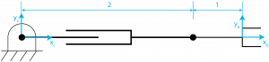
4. Frame {0} and frame {1} are along with their respective vectors are shown in the below illustration. Please note that all the axes are parallel ([latex]z_0 || y_1, x_0 || x_1, y_0 || z_1[/latex]). Find the position vector, p0, and the homogeneous transformation matrix, [latex]H_1^0[/latex]
![]()
Answer:
[latex]R_0^1=R_{x,90°}=\begin{bmatrix} 1 & 0 & 0 \\ 0 & c_90 & -s_90 \\ 0 & s_90 & c_90 \end{bmatrix} = \begin{bmatrix} 1 & 0 & 0 \\ 0 & 0 & -1 \\ 0 & 1 & 0 \end{bmatrix}[/latex]
[latex]p^0 = R_1^0 p ^1 + d_1^0 = \begin{bmatrix} 0 \\ 2 \\ 2 \end{bmatrix}[/latex]
[latex]H_1^0=\begin{bmatrix} R_1^0 & d_1^0 \\ 0 & 1 \end{bmatrix} = \begin{bmatrix} 1 & 0 & 0 & 0 \\ 0 & 0 & -1 & 3 \\ 0 & 1 & 0 & 1 \\ 0 & 0 & 0 & 1 \end{bmatrix}[/latex]
5. Derive the forward kinematics equations using the DH Convention for the cylindrical robot shown below.

Answer:
| Link | ai | αi | di | θi |
| 1 | 0 | 0° | d1 | θ1* |
| 2 | 0 | -90° | d2 | 0 |
| 3 | 0 | 0° | d3 | 0 |
| [latex]A_1=\begin{bmatrix} c_1 & -s_1 & 0 & 0 \\ s_1 & c_1 & 0 & 0 \\ 0 & 0 & 1 & d_1 \\ 0 & 0 & 0 & 1 \end{bmatrix}[/latex] | [latex]A_2=\begin{bmatrix} 1 & 0 & 0 & 0 \\ 0 & 0 & 1 & 0 \\ 0 & -1 & 0 & d_2 \\ 0 & 0 & 0 & 1 \end{bmatrix}[/latex] | [latex]A_3=\begin{bmatrix} 1 & 0 & 0 & 0 \\ 0 & 1 & 0 & 0 \\ 0 & 0 & 1 & d_3 \\ 0 & 0 & 0 & 1 \end{bmatrix}[/latex] |
[latex]T_3^0=A_1A_2A_3=\begin{bmatrix} c_1 & 0 & -s_1 & -d_3 s_1 \\ s_1 & 0 & c_1 & d_3 c_1 \\ 0 & -1 & 0 & d_1 + d_2 \\ 0 & 0 & 0 & 1 \end{bmatrix}[/latex]
6. Derive the forward kinematics equation using the DH Convention for the following robot.

Answer:
| Link | ai | αi | di | θi |
| 1 | 0 | 90° | a1 | θ1*+90° |
| 2 | 0 | 0° | a2+a3+d2 | 0 |
[latex]A_1=\begin{bmatrix} c(\theta_1 + 90°) & 0 & s(\theta_1+90°) \cdot 1 & 0 \\ s(\theta_1 + 90°) & 0 & c(\theta_1+90°) \cdot 1 & 0 \\ 0 & 1 & 0 & a_1 \\ 0 & 0 & 0 & 1 \end{bmatrix} = \begin{bmatrix} -s_1 & 0 & c_1 & 0 \\ c_1 & 0 & s_1 & 0 \\ 0 & 1 & 0 & a_1 \\ 0 & 0 & 0 & 1 \end{bmatrix}[/latex]
[latex]A_2=\begin{bmatrix} 1 & 0 & 0 & 0 \\ 0 & 1 & 0 & 0 \\ 0 & 0 & 1 & a_2 + a_3 + d_2 \\ 0 & 0 & 0 & 1 \end{bmatrix}[/latex]
[latex]T_2^0 = A_1 A_2 = \begin{bmatrix} -s_1 & 0 & c_1 & (a_2 + a_3 + d_2) c_1 \\ c_1 & 0 & s_1 & (a_2 + a_3 + d_2)s_1 \\ 0 & 1 & 0 & a_1 \\ 0 & 0 & 0 & 1 \end{bmatrix}[/latex]
7. Find the angular and linear velocity for the following illustration.

Answer:
| [latex]S_w=\begin{bmatrix} 0 \\ 0 \\ 1 \end{bmatrix}[/latex] | [latex]S_v=\begin{bmatrix} \frac{-2}{sqrt{2}} \\ \frac{-2}{sqrt{2}} \\ 0[/latex] |
8. Find the angular and linear velocity for the following illustration.

Answer:
| [latex]S_w=\begin{bmatrix} 0 \\ - 1 \\ 0 \end{bmatrix}[/latex] | [latex]S_v = \begin{bmatrix} 0 \\ 0 \\ 0 \end{bmatrix}[/latex] |
9. Consider the following robot in its’ zero-frame orientation. Derive the forward kinematics using Screw Theory using either the space or end effector frame.
Answer:
[latex]M=\begin{bmatrix}0 & -1 & 0 & 19 \\ -1 & 0 & 0 & 0 \\ 0 & 0 & -1 & -3 \\ 0 & 0 & 0 & 1 \end{bmatrix}[/latex]
Space Frame-
| [latex]S_1=\begin{bmatrix} 0 \\ 0 \\ 1 \\ 0 \\ 0 \\ 0 \end{bmatrix}[/latex] | [latex]S_2=\begin{bmatrix} 0 \\ 0 \\ 1 \\ 0 \\ -10 \\ 0 \end{bmatrix}[/latex] | [latex]S_3=\begin{bmatrix} 0 \\ 0 \\ 1 \\ 0 \\ -19 \\ 0 \end{bmatrix}[/latex] | [latex]S_4=\begin{bmatrix} 0 \\ 0 \\ 0 \\ 0 \\ 0 \\ 1 \end{bmatrix}[/latex] |
End Effector Frame-
| [latex]B_1=\begin{bmatrix} 0 \\ 0 \\ -1 \\ -19 \\ 0 \\ 0 \end{bmatrix}[/latex] | [latex]B_2=\begin{bmatrix} 0 \\ 0 \\ -1 \\ -9 \\ 0 \\ 0 \end{bmatrix}[/latex] | [latex]B_3=\begin{bmatrix} 0 \\ 0 \\ -1 \\ 0 \\ 0 \\ 0 \end{bmatrix}[/latex] | [latex]B_4=\begin{bmatrix} 0 \\ 0 \\ 0 \\ 0 \\ 0 \\ -1 \end{bmatrix}[/latex] |
Simulation and Animation
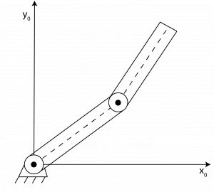
Let’s look back at the two-link planar manipulator used with the trigonometry method. Below is the basic illustration of it.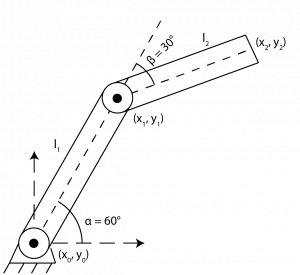
The simulation and code for this example can be found here.
References[1] Ben-Ari, M., & Mondada, F. (2017). Kinematics of a Robot Manipulator. In M. Ben-Ari, & F. Mondada, Elements of Robotics (pp. 267-291). Springer, Cham.
[2] Krishna, S. (n.d.). Forward Kinematics. Retrieved from Robotics Learning: https://www.rosroboticslearning.com/forward-kinematics
[3] Lynch, K. M., & Park, F. C. (n.d.). Video Supplements for Modern Robotics. Retrieved from Northwestern: https://modernrobotics.northwestern.edu/nu-gm-book-resource/forward-kinematics-example/#department
[4] Robot Modeling and Control. (2006). Wiley.
[5] Wang, D. Y. (2021). Fall 2021 ME8930 Lectures. Zoom.
