
6 Trajectory Generation
Ananya Rao
CHAPTER 6 TRAJECTORY GENERATION
OUTLINE
6.1 Introduction
6.2 Trajectory Generation Approaches
6.2.1 Point to Point Trajectory Planning
6.2.2 Trajectory Planning Via Polynomial Points
6.2.3 Time-optimal Time Scaling
6.3 Trajectory Profiles
6.3.1 Straight line profile
6.3.2 Polynomial profile
6.3.3 Bang-bang acceleration profile
6.3.4 Trapezoidal acceleration profile
6.4 Trajectory Generation Algorithms
6.4.1 Minimum Execution Time Algorithm
6.4.2 Minimum Energy Consumption Algorithm
6.4.3 Minimum Jerk Algorithm
6.5 Summary
6.6 Practice Questions
Simulation and Animation
6.1 Introduction
For the robot to move from origin to destination, a specific path has to be defined which the robot can take. This specified path consists of a sequence of points which can either be defined in the task space or joint space of the robot. The end effector or the base joint variables are defined as a function of time. Trajectory generation deals with the generation of the specified path which the robot tracks in order to move from start to the end. Trajectory generation of the robot in joint space and in task space they can be classified as follows:
- Trajectory generation in joint space:
- Generating trajectory between two points following free path between them
- Generating trajectory between two points by including a sequence of intermediate points.
- Trajectory generation in task space:
- Generating trajectory between two points by including straight line segment (constrained) path between them.
- Generating trajectory between two points with constrained path between the via points.
Block diagram for the two approaches of trajectory generation is given in below.

Figure 6.1 Trajectory generation in joint space

Figure 6.2 Trajectory generation in task space
Depending on whether the constraints are defined in joint or task space, a relevant trajectory generation approach is taken.
6.2 Trajectory Generation Approaches
In this section we’ll discuss different approaches for generating the trajectory of each joint of the robot. The subsections give a detailed description of what those approaches are and how it is achieved.
6.2.1 Point to Point Trajectory Planning
Configuration of the robot is defined as a function of time, this is known as trajectory.
[latex]θ(t),tϵ[0,T] (6.1)[/latex]

Figure 6.3 Trajectory of the robot represented in the C-space
A path is a curve equation written as a function of s (path parameter) in the configuration space.
[latex]θ(s),sϵ[0,1] (6.2)[/latex]
The path function mapped to the time domain gives the trajectory. This mapping is known as time scaling which controls how fast the path is being followed.
[latex]s:[0,T]→[0,1] (6.3)[/latex]
[latex]θ ̇=dθ/ds s ̇ (6.4)[/latex]
[latex]θ ̈=dθ/ds s ̈+(d^2 θ)/ds s ̇^2 (6.5)[/latex]
For the system to be valid [latex]θ(s) and s(t)[/latex] must exist and be double differentiable. Considering a straight line path starting from [latex]θ_start[/latex] and ending in [latex]θ_end[/latex] is given by:
[latex]θ(s)= θ_start+s(θ_end-θ_start ),sϵ[0,1] (6.6)[/latex]
[latex]dθ/ds=θ_end-θ_start; (d^2 θ)/ds=0 (6.7)[/latex]
where [latex]θ_(i,min) ≤ θ_(i )≤ θ_(i,max)[/latex] for each joint.
It is important to note that the straight line in joint space is not equal to straight line in task space.
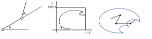
Figure 6.4 Straight line trajectory in different spaces.
6.2.2 Trajectory Planning Via Polynomial Points
This section explains about trajectory generation when additional points, known as via points are introduced in between the starting and end points. This method is often employed to evade objects and hence avoid collision. A polynomial can be found which each via points can satisfy but wouldn’t be feasible as the number of points increase. Hence the trajectory is split into different section to ease the computation load.
Linear interpolation with continuous acceleration blends
This method can be used in both joint and task space. Straight line segments with constant velocity are used to connect the via points. These line segments are connected using continuous acceleration motions. A smooth trajectory can be generated by not stopping at the via points. To achieve this, the segments at k-1 and k are connected by a blend. Time taken in the blend region at point k is 2Tk . Blend region has maximum acceleration at each joint. Hence the blend time for each point is given by:
[latex]T_(k,j)=3/4 |(q ̇_j^k-q ̇_j^(k-1))/k_(a,j) |for k=2,…,m-1;j=1,…,n (6.8)[/latex]
The joints are synchronized at region of blends around initial and final points.
[latex]T_(k,j)=τ^'/2 (6.9)[/latex]
If [latex]q_(j,a)^k[/latex] and [latex]q_(j,b)^k[/latex] are the positions of joint at the beginning and the end then,
[latex]q_(j,a)^k=q_j^k-T_(k,j) q ̇_j^(k-1) q_(j,b)^k=q_j^k-T_(k,j) q ̇_j^k (6.10)[/latex]
Equation of motion of joint j at segment k is
[latex]q_j (t)=(t-t_k-T_k ) q ̇_j^k+q_j^k for t_k+2T_k≤t≤t_(k+1) (6.11)[/latex]
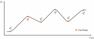
Figure 6.5 Linear interpolation with continuous acceleration blends
This method can be modified by replacing linear interpolation with cubic spline interpolation with continuity of velocity and acceleration. Furthermore, the generated path can be decoupled from history of time along the path with which velocity could be modified run-time while tracking the desired path.
6.2.3 Time-optimal Time Scaling
[latex]θ ̇=s ̇(θ_end-θ_start ); θ ̈=s ̈(θ_end-θ_start) (6.12)[/latex]
Consider the n-th order polynomial given by:
[latex]q(t)=a_n t^n+a_(n-1) t^(n-1)+⋯+〖 a〗_1 t+a_0 (6.13) Where, t→Time and a_i (i=0,1,2,…,n)→polynomial coefficients[/latex]
In order to reduce the higher order terms the joint motion is divided into three parts consisting of four key points. They are, initial point, transition point from acceleration to constant velocity, transition point from constant velocity to deceleration and the end point. Firstly part starts with acceleration followed by constant velocity phase and finally the deceleration phase. Initial and final velocity and accelerations are set to zero. Acceleration must be set to zero in all the four key points. Hence, the acceleration profile can be written as:
[latex](q_a ) ̈(t)=bt^k (t-t_1 )^l (6.14) where, b→coefficinet t_1→transition point from acceleration to constant velocity k→multiplicity of root 0 l→multiplicity of root t_1[/latex]
Similarly, the deceleration profile can be written as:
[latex](q_a ) ̈(t)=c(t-t_2 )^m [(t-t_2 )-(t_3-t_2 )]^p where, c→coefficinet t_2→transition point from constant velocity to deceleration t_3→time at the end point m→multiplicity of root t_2 p→multiplicity of root t_3[/latex]
Jerk associated with the deceleration part of the trajectory profile is obtained by differentiation of equation (6.10) with respect to time.
[latex](q_a ) ̈(t)=b(kt+lt-kt_1 ) t^(k-1) (t-t_1 )^(l-1) (6.16)[/latex]
Jerk associated with the deceleration part of the trajectory profile is obtained by differentiating equation (7.11) with respect to time.
[latex](q_d ) ̈(t)=c(mt+pt-mt_3-pt_2 )(〖t-t_2)〗^(m-1) (t-t_3 )^(p-1) (7.17)[/latex]
Jerk is set to zero in all four key points in order to ensure the continuity of jerk. Joint velocity is given by:
[latex]q ̇(t)={(b(1/5 t^5-t/2 t_1 t^4+1/3 t_1^2 t^3 for (0≤t≤t_0)@v_0 for (t_1≤t≤t_2 )@v_0+c[1/5 t^5-1/2 (t_2 〖+t〗_3 ) t^4+1/3 (t_2^2+4t_2 t_3+t_3^2 ) t^3-(t_2 t_3^2+t_2^2 t_3 ) t^2+t_2^2 t_3^2 t]@for (t_2≤t≤t_3))┤ (6.18) [/latex]
6.3 Trajectory Profiles
Talks about the different types of profiles in trajectory generation. The subsection elaborates on the same.
A path is a pure geometric description of the sequence of configurations that the robot takes from rest or start to goal position. In general, a path is a function [latex]θ∶[0,1]→ ξ[/latex] that maps a scalar path parameter to a point in configuration space [latex]ξ. s=0 and s=1[/latex] are the start and end of the path respectively.
A path is defined as [latex]p(s)=(x(s),y(s),z(s))[/latex] with the motion law. [latex]s=s(t)[/latex]Based on this definition, we can compute the velocity [latex]p ̇(s)=dp/ds s ̇(t)[/latex] and acceleration [latex]p ̈(s)=dp/ds s ̈(t)+(d^2 p)/ds s ̇(t) .[/latex]. Hence, based on the motion law s(t), we can generate different trajectory profiles to satisfy various applications such as pick and place, maneuvering etc.
6.3.1 Straight line profile
One way to determine the configuration sequence to take a straight-line path from start to goal. A straight line in configuration space does not lead to a straight-line motion in the end effector space (consider for example, a straight-line path from [latex]θ_start[/latex] to [latex]θ_end[/latex] in joint space where represents the joint angle). In fact, a straight line in Euclidean space maps to a screw motion in SE(3) as shown in Figure 7.6

Figure 6.6: A straight line end effector path from point A to B of a 2-link planar robotic arm leads to a screw motion of the joint parameters α and β
A straight-line motion in joint space is given by:
[latex]θ(s)= θ_start+s(θ_end-θ_start)[/latex]
A straight-line motion in task space is given by:
[latex]x(s)= x_start+s(x_end-x_start)[/latex]
We can design a straight-line path in task space by using two approaches
Approach 1:
By using the straight-line equation,
[latex]x(s)= x_start+s(x_end-x_start)[/latex]
and computing the joint space path [latex]θ(p)[/latex] using inverse kinematics.
Approach 2:
By designing a screw motion in SE(3) which leads to a straight line in task space. Let the screw path by defined by X(p) with constant twist with the following boundary conditions.
[latex]X(0)=T_start ; X(1)=T_end[/latex]
[latex]where T_start and T_end[/latex] are the start and end times respectively.
Then, we can write X(p) as,
[latex]X(s)=T_start exp(log(T_start^(-1) T_end )p)[/latex]
The transnational and rotational parts of X(p) are given by,
[latex]z(s)=z_start+s(z_end-z_start )[/latex]
[latex]R(s)=R_start exp(log(R_start^T R_end )p)[/latex]
One can define the motion law s(t) to ensure a smooth motion along [latex]θ(s)[/latex] based on velocity and acceleration constraints. Here maps from [latex][0,T]→[0,1].[/latex] For pick and place applications, we want zero velocities at the start and end positions. This translates to the following boundary conditions.
[latex]s(0)=0;s(T)=1;s ̇(0)=0;s ̇(T)=0[/latex]
6.3.2 Polynomial profile
A cubic polynomial of the form [latex]s(t)=a_0 t+a_1 t+a_2 t^2+a_3 t^3[/latex] can satisfy the above constraints and lead to a smooth profile with max joint velocity at [latex]t=T/2[/latex] and max joint acceleration and deceleration at t=0 and t=T respectively as shown in Figure 6.7

Figure 6.7 (a) position profile (b) velocity profile (c) acceleration profile
In some situations, having zero acceleration at start and end positions is desirable. In this case, a quintic (5th order) polynomial [latex]s(t)=a_0 t+a_1 t+a_2 t^2+a_3 t^3+a_4 t^4+a_5 t^5[/latex] can be used as the motion law with the following boundary conditions:
[latex]s(0)=0;s(T)=1;s ̇(0)=0;s ̇(T)=0; s ̈(0)=0;s ̈(T)=0[/latex]
The coefficients of these polynomials can be solved uniquely based on the boundary conditions leading to an acceleration profile with zero acceleration at the start and end positions as shown in Figure 6.8

Figure 6.8: (a) position profile starting from [latex]s(t)=0[/latex] and terminating at [latex]s(T)=1[/latex] (b) velocity profile max velocity [latex]s ̇(T/2)=15/2T[/latex] (c) acceleration profile max acceleration [latex]s ̈(3T/4)= -10/(T^2 √3)[/latex]
6.3.3 Bang-bang acceleration profile
This profile consists of a discontinuous acceleration profile defined by a constant acceleration phase till [latex]t=T/2[/latex] followed by a constant deceleration phase till [latex]t=T[/latex] as shown in Figure 6.9

Figure 6.91 Bang-bang acceleration profile with position profile starting from [latex]s(t)=0[/latex] and terminating at [latex]s(T)=1[/latex] , velocity profile with [latex]s ̇(0)=s ̇(T)=0[/latex] and max velocity [latex]s ̇(T/2)=2/T[/latex] and acceleration profile with constant acceleration and deceleration phase of [latex]s ̈(t)=4/T^2[/latex]
Figure 6.92 Trapezoidal acceleration profile with position profile starting from [latex]s(t)=0[/latex] and terminating at [latex]s(T)=1[/latex] , velocity profile with [latex]s ̇(0)=s ̇(T)=0[/latex] and [latex]s ̇(t_j )=constant[/latex] and acceleration profile with a constant acceleration and deceleration phase of [latex]s ̈(t_j )=constant[/latex]
6.3.4 Trapezoidal acceleration profile
Adding a constant velocity phase to the bang-bang acceleration profile at the point when velocity reaches max leads to saturation in acceleration phase as shown in Figure 6.10. This profile also leads to minimum travelling time which makes it suitable for certain measuring tasks with fast transition time requirements.
6.4 Trajectory Generation Algorithms
There are different algorithms used to generate the trajectory. These algorithms are explained in detail in the below subsections.
6.4.1 Minimum Execution Time Algorithm
This section aims at introducing trajectory generation algorithm which aim to minimize travel time from initial configuration [latex](q^i )[/latex] to find configuration [latex](q^f )[/latex] without defying velocity and acceleration constraints. Minimum travel time occurs when both velocity and acceleration are at its maximum value. Thereby, the global minimum time [latex]t_f[/latex] is equal to the largest minimum time given by:
[latex]t_f=max(t_f1,… ,t_fn (6.23)[/latex]
Based on the values of maximum velocity and maximum acceleration for different interpolation function, minimum travel time is given by:
| Interpolation function | Minimum time |
| Linear interpolation | [latex]t_fj= (|D_j |)/k_vj[/latex] |
| Cubic polynomial | [latex]t_fj=max[ 3|D_j |/〖2k〗_vj ,√(6|D_j |/k_aj )][/latex] |
| Ouintic polynomial | [latex]t_fj=max[ 15|D_j |/〖8k〗_vj ,√(10|D_j |/〖√3 k〗_aj )][/latex] |
| Bang-bang profile | [latex]t_fj=max[ 2|D_j |/k_vj ,2√(|D_j |/k_aj )][/latex] |
Table 6.1 Minimum traveling time
Time-Optimal Time Scaling
This section focuses on minimizing the time of travel. This will eventually increase the productivity of the robot. General equation of Dynamics of the robot is:
[latex]m(θ) θ ̈+(θ^T ) ̇Γ(θ) θ ̇+g(θ)= τ (6.24)[/latex]
Plugging equations (6.4) and (6.5) in equation (6.22) we get
[latex](m(θ(s)) dθ/ds) s ̈ +(m(θ(s)) (d^2 θ)/ds+(dθ/ds)^T Γ θ(s) dθ/ds) s ̇^2+g(θ(s))= τ (7.25)[/latex]
[latex]m(s) s ̈+c(s) s ̇^2+g(s)= τ (6.26)[/latex]
Equation (7.26) gives the dynamics of the robot on the path. Limit of the actuator is given by:
[latex]T_i^min (s,s ̇ )≤T_i≤T_i^max (s,s ̇ ) (6.27)[/latex]
[latex]T_i^min (s,s ̇ )≤m_i (s) s ̈+c_i (s) s ̇^2+g_i (s)≤T_i^max (s,s ̇ ) (6.28)[/latex]
[latex]if m_i (s)>0,L_i (s,s ̇ )=(T_i^min (s,s ̇ )-c(s) s ̇^2-g(s))/(m_i (s)) (6.29)[/latex]
[latex]U_i (s,s ̇ )= (T_i^max (s,s ̇ )-c(s) s ̇^2-g(s))/(m_i (s)) (6.30)[/latex]
[latex]L(s,s ̇ )=max┬i〖L_i (s,s ̇ ) and U(s,s ̇ )= min┬i〖U_i (s,s ̇)〗 〗 (6.31)[/latex]
Then for the robot to stay on the path,
[latex]L(s,s ̇ )≤s ̈≤U(s,s ̇) (6.32)[/latex]
If [latex]L(s,s ̇ ) >U(s,s ̇)[/latex] then the robot digresses from the path.
Consider a target (to the motion) vector at [latex]state(s,s ̇)[/latex]. The vertical component of acceleration can be [latex]U(s,s ̇)[/latex] or [latex]L(s,s ̇ ).[/latex].
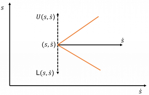
Figure 6.10
The resultant vectors from the feasible motion cone. For a given s if [latex]s ̇[/latex] keeps increasing it hits a point where L=U. The locus of this point for different [latex](s,s ̇ )[/latex] gives a speed limit curve. Integrating the minimum acceleration L backward from end state till s becomes zero followed by forward integration of max acceleration from initial state to the velocity limit curve. The two curves will meet at a point thus forming the optimal time scaling. Repeating the same for different states [latex](s,s ̇)[/latex] will give the time-optimal time scaling trajectory. This time scaling ensures max velocity while keeping the trajectory feasible for actuators.
6.4.2 Minimum Energy Consumption Algorithm
This section talks about optimal energy consumption exploits probabilistic road maps that helps employing the best geometrical path along which the velocity and acceleration of the robot are maximum. Within the set tasks of the robot, a collision free trajectory is generated by using probabilistic road maps. In order to achieve this a set of points in the robot environment is considered. The amount of energy that will be consumed is calculated for all the points in the vicinity. The trajectory with the lowest energy consumption is set as the nearest points. A map is then used to find the minimum energy trajectories between different points for any given task. Minimum energy trajectories are identified using Dijkstra algorithm.
6.4.3 Minimum Jerk Algorithm
This algorithm is employed to generate smooth-optimal trajectories. Due to higher dimension of the state space computation loads are increased which makes optimal control complicated. Based on properties of differential flatness, the behavior of the system outputs can be determined.
Step 1: flat outputs are chosen, so the system can be mapped to a lower dimensional output space. Cost function, boundary conditions are also mapped to this lower dimensional output space.
Step 2: Choose suitable basis function to parameterize the system output.
Step 3: After parameterize, the system equations are solved using B-splines to minimize the cost function and also to satisfy the boundary conditions.
Step 4: The obtained flat output trajectories have minimum jerk.
6.5 Summary
This chapter talks about trajectory generation which is an indication of a robot’s position, velocity and acceleration as a function of time for each way point in the specified path. Trajectory = (specified path + time scaling function) Cubic polynomial method is one of the most common approaches to obtain a trajectory. Higher order polynomials can give a more accurate estimate of co-efficient and hence a better trajectory can be generated. Trapezoidal method is the other, most sort after method to generate a trajectory. In spite of compromising on the smoothness of the curve. It can implement joint velocity and acceleration limits with much more ease. Hence it can generate trajectories with constraints on jerk, velocity and time limits.
6.6 Practice Questions
- What are the advantages and disadvantages of calculating trajectory in operating space and joint space.
Operating Space
Advantages:- Easy to derive a collision free path.
Disadvantages:
- Inverse kinematics imparts expensive load computationally
Determining time path is not straight forward
Joint Space
Advantages:
- It is easy to compute inverse kinematics as the calculation need not have to be repeated.
- Easy to implement joint angle and velocity constraints.
Disadvantages:
- Difficult to implement obstacle avoidance.
- A single link manipulator with a revolt joint stopping at [latex]θ=30°[/latex]. It is desired to move the joint in a smooth manner to [latex]θ=60°[/latex] in 5 seconds. Find the coefficients of a cubic that can implement this motion and bring the manipulator to rest at the goal position.
Solution
Given, [latex]θ_0=30°, θ_f=60°, t_f=5s[/latex]
[latex]a_0=θ_0,a_1=0,a_2=3/(t_f^2 ) (θ_f-θ_0 ),a_3=-2/(t_f^3 ) (θ_f-θ_0 )[/latex]
[latex]a_0=30°, a_1=0 , a_2=3/125 (60-30)=0.72 , a_3= -2/125 (60-30)=-0.48[/latex]
Joint position: [latex]θ(t)=30+0.72t^2-0.48t^3[/latex]
Joint velocity along this path: [latex]θ ̇(t)=1.44t(1-t)[/latex]
Joint acceleration along this path: [latex]θ ̈(t)=1.44(1-2t)[/latex] - Write a code to generate a plot for position, velocity and acceleration for the equations obtained in problem 2.
Solution:t = 0:0.01:5;theta_t = 30 + 0.72*t*t – 0.48*t*t*t;theta_dot_t = 1.44*t – 1.44*t*t;theta_dot_dot_t = 1.44 – 2.88*t;subplot(3,1,1);plot(t,theta_t); grid on;ylabel(‘position (degree)’);subplot (3,1,2);plot(t,theta_dot_t); grid on;
ylabel (‘velocity (degree/s)’);
subplot (3,1,3);
plot(t,theta_dot_dot_t); grid on;
ylabel (‘acceleration (degree/s^2)’);
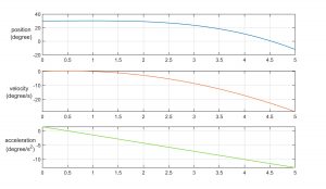
Figure 6.11: position, velocity and acceleration plots for the given trajectory - Solve the coefficients of two cubic that are connected in a two-segment spline with continuous velocity and acceleration at the via point. Given: initial angle [latex]θ_0[/latex], via point [latex]θ_v[/latex], goal point [latex]θ_g[/latex].
Solution:
[latex]θ_1 (t)=a_10+a_11 t+a_12 t^2+a_13 t^3[/latex]
[latex]θ_2 (t)=a_20+a_21 t+a_22 t^2+a_23 t^3[/latex]Angular constraints for first cubic:Initial position [latex]θ_0=a_10[/latex]
End position [latex]θ_v=a_10+a_11 t_f1+a_12 t_f1^2+a_13 t_f1^3[/latex]Angular constraints for second cubic:Initial position [latex]θ_v=a_20[/latex]
End position [latex]θ_g=a_20+a_21 t_f2+a_22 t_f2^2+a_23 t_f2^3[/latex] - Solve for the coefficient of two cubic that are connected in a two-segment spline with continuous velocity and acceleration at the via point.
Solution:
[latex]θ_1 (t)=a_10+a_11 t+a_12 t^2+a_13 t^3[/latex]
[latex]θ_2 (t)=a_20+a_21 t+a_22 t^2+a_23 t^3[/latex]
Angular velocity constraint for first cubic: Start from rest: [latex]a_11=0[/latex]
Angular velocity constraint for second cubic: zero at rest: [latex]0=a_21+2a_22 t_f2+3a_23 t_f2^2[/latex]
Equating the two equations:
[latex]a_11+2a_12 t_f1+3a_13 t_f1^2=a_21[/latex]
[latex]2a_12+6a_13 t_f1=2a_22[/latex]
[latex]θ_0=a_10; θ_v=a_10+a_11 t_f1+a_12 t_f1^2+a_13 t_f1^2;[/latex]
[latex]θ_v=a_20; θ_g=a_20+a_21 t_f2+a_22 t_f2^2+a_23 t_f2^2;[/latex]
[latex]a_11=0; a_21+2a_22 t_f2+3a_23 t_f2^2=0;[/latex]
[latex]a_11+2a_12 t_f1+3a_13 t_f1^2=a_21;[/latex]
[latex]2a_12+6a_13 t_f1=2a_22;[/latex]
Consider [latex]t_f=t_f1=t_f2:[/latex]
[latex]a_10=θ_0; a_11=0;[/latex]
[latex]a_12=(〖12θ〗_v-3θ_g-θ_0)/(4t_f1^3 ) ; a_13=(〖-8θ〗_v+3θ_g+5θ_0)/(4t_f1^2 ) ;[/latex]
[latex]a_20=θ_v ; a_21=(3θ_g-3θ_0 0)/(4t_f ) ;[/latex]
[latex]a_22=(-12θ_v+6θ_g+6θ_0)/(4t_f^2 ) ; a_23=(8θ_v-5θ_g-3θ_0)/(4t_f^3 )[/latex] - Single link manipulator with a revolt joint stopping at [latex]θ_0=30°[/latex] and [latex]θ_f=60° t=3s[/latex].
Solve the problem for high acceleration and low acceleration of a linear path with parabolic blends.
Solution:Position, velocity and acceleration profiles for linear interpolation with parabolic blends and find [latex]t_b[/latex] and [latex]θ_b[/latex]
Given: [latex]θ_0=30° and θ_f=60° t_f=3s[/latex]
[latex]t_b=t_f/2-√(〖t_f〗^2 θ ̈^2-4θ ̈(θ_f-θ_0 ) )/(2θ ̈ ) -→ t_b=3/2-√(9θ ̈^2-4θ ̈(60-30))/(2θ ̈ )[/latex]
[latex]θ ̈≥4(θ_f-θ_0 )/〖t_f〗^2 -→ θ ̈≥4(60)/9 → θ ̈≥26.67[/latex]
For [latex]θ ̈_max=30 (let) → t_b=1s[/latex]
for [latex]θ ̈_min=26.67 → t_b=1.483s[/latex] - Way-points of a certain trajectory given in degrees are: 10, 40, 20,10. Time taken for these segments are 2, 1 and 3 seconds respectively. Acceleration is 50 [latex]degrees/s^2[/latex] . Calculate velocity, blend times, linear times for all segments and sketch the trajectory.
Solution:
Segment 1
Formula:
[latex]Θ ̈=SGN(Θ_2-Θ_1 )|Θ ̈_1 |, t_1=t_d12-√(t_d12^2-(2(Θ_2-Θ_1))/Θ ̈_1 ), Θ ̇_12= (Θ_2-Θ_1)/(t_d12-(1t_1)/2) ,[/latex]
[latex]Θ ̈_1=50deg/s^2 ,[/latex]
[latex]t_1=2-√(4-2(40-10)/(50 ))=0.3267 ; t_2=1-√(1+((20-40)*2)/50)=0.553s ;[/latex]
[latex]t_3=(-3.371-(-27.643))/50=0.48544s ; t_4=3-√(9+((10-20)*2)/50)=0.067s ;[/latex]
[latex]Θ ̇_12= (40-10)/(2-0.5*0.3267)=16.334 °/s ; Θ ̇_23= (20-40)/(1-0.5*0.553)=-27.643 °/s ;[/latex]
[latex]Θ ̇_34= (10-20)/(3-0.5*0.067)=-3.371 °/s ;[/latex]
[latex]t_23=1-1/2 (0.553+0.48544)=0.481s ; t_34=3-0.067-1/2 (0.48544)=2.690s ;[/latex] - Generate a cubic polynomial trajectory. The robot starts at rest from a horizontal position. The final position of the robot is as given in the figure below. Time taken to reach the final position is 8s. Plot [latex]θ(t),θ ̇(t),θ ̈(t).[/latex] Time interval remains constant for all the joints.

Figure 6.12 : Final position of the three-link robotic arm
Solution:
At [latex]t=0,θ_1=0,θ_2=0,θ_3=0;[/latex]
From the figure, final position is [latex]θ_1=90,θ_2=-90,θ_3=-90[/latex]
[latex]θ ̇_1=0,θ ̇_2=0,θ ̇_3=0 at t=8s[/latex]
[latex]θ_1 (t)=a_0+a_1 t+a_2 t^2+a_3 t^3[/latex]
[latex]BC: θ_1 (0)=0; θ_1 (8)=π/2; θ ̇_1 (0)=0;θ ̇_1 (8)=0;[/latex]
Substituting the boundary conditions we get, [latex]a_0=0; a_1=0;a_2=3π/128;a_3=(-π)/512[/latex]
Therefore,
[latex]θ_1 (t)=〖3π/128 t〗^2+(-π)/512 t^3 ; θ ̇_1 (t)= 3π/64 t-3π/512 t^2 ; θ ̈_1 (t)=3π/64-3π/256 t[/latex]
[latex]θ_2 (t)=a_0+a_1 t+a_2 t^2+a_3 t^3[/latex]
[latex]BC: θ_2 (0)=0; θ_2 (8)=-π/2; θ ̇_2 (0)=0;θ ̇_2 (8)=0;[/latex]
Substituting the boundary conditions we get, [latex]a_0=0; a_1=0;a_2=(-3π)/128;a_3=π/512[/latex]
Therefore,[latex]θ_2 (t)=〖-3π/128 t〗^2+π/512 t^3 ; θ ̇_2 (t)= -3π/64 t+3π/512 t^2 ; θ ̈_2 (t)=-3π/64+3π/256 t ;[/latex][latex]θ_3 (t)=a_0+a_1 t+a_2 t^2+a_3 t^3[/latex]
[latex]BC: θ_3 (0)=0; θ_3 (8)=-π/2; θ ̇_3 (0)=0;θ ̇_3 (8)=0;[/latex]
Substituting the boundary conditions we get, [latex]a_0=0; a_1=0;a_2=(-3π)/128;a_3=π/512[/latex]
Therefore,
[latex]θ_3 (t)=〖-3π/128 t〗^2+π/512 t^3 ; θ ̇_3 (t)= -3π/64 t+3π/512 t^2 ; θ ̈_3 (t)=-3π/64+3π/256 t ;[/latex]
Simulation and Animation
Taking the example of a three-link robotic arm, a trajectory is generated for the movement of the end effector from base position to a target position. The simulation video for this and the related files can be accessed here.
 Figure 6.13 :Three-link robotic arm considered for trajectory generation simulation
6.6 References
This section will include all the codes for defining and running the simulation.
- Spong, M.W., Hutchinson, S. and Vidyasagar, M., 2020. Robot modeling and control. John Wiley & Sons.
- Gasparetto, A., Boscariol, P., Lanzutti, A. and Vidoni, R., 2015. Path planning and trajectory planning algorithms: A general overview. Motion and operation planning of robotic systems, pp.3-27.
- Ragaglia, M., Zanchettin, A. M., & Rocco, P. (2018). Trajectory generation algorithm for safe human-robot collaboration based on multiple depth sensor measurements. Mechatronics, 55, 267-281.
- Yu, J., Cai, Z., & Wang, Y. (2014, August). Minimum jerk trajectory generation of a quadrotor based on the differential flatness. In Proceedings of 2014 IEEE Chinese guidance, navigation and control conference(pp. 832-837). IEEE.
- Pellegrinelli, S., Borgia, S., Pedrocchi, N., Villagrossi, E., Bianchi, G., & Tosatti, L. M. (2015). Minimization of the energy consumption in motion planning for single-robot tasks. Procedia Cirp, 29, 354-359.
