7.1.1 Simulation setup in copeliasim

In order to show how various offline motion planning algorithms works, I am also going to use the copeliasim simulation for representing these offline motion planning.  I will be using Pioneer 3-DX as the robot in the copeliasim environment as shown in figure 7.1. In the simulation, a camera is added, which basically shows the whole environment as an image as shown in figure 7.2. The main reason for the camera usage is to visualize these offline motion planning algorithms, which is understandable by everyone. The same simulation setup is used for all offline motion planning algorithms, in order to show the difference between these algorithms. 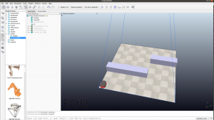Fig 7.1: copeliasim Simulation setup for offline motion planning

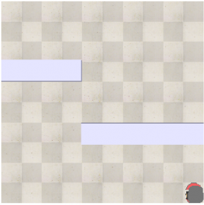
Fig 7.2: Camera output from the simulation for visualization of offline motion planning

7.2 Grid-based Methods

Grid-based motion planning is a technique, where the collision-free space is divided into smaller cells, where the graph node is at the center of the cell. The individual cell can be of any shape ( square, triangle, trapezoid, etc)[1]. A square grid is often used thanks to its simplicity without loss of generality. Every grid-based motion planning algorithm contains the following elements:

• Finite State Space: It is a set of all possible states which are collision-free. Here each state is considered as a node, which is very helpful to understand grid-based motion planning.
• Action: It is transitioning from the current cell to neighboring cells.
• Transition Function: This is a function that moves to a neighboring cell by performing an action from the parent cell.
• Cost Function: It is the cost to transition from the current cell to the neighboring cell using a particular action.

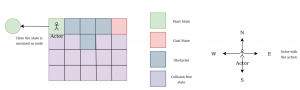
Fig 7.3: Representation of state (node), action and its representation

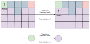
Fig 7.4: Transition from the current cell to a neighboring node in state and node representation using a cost function

Here, grid-based motion planning is the sequence of actions, which is cost-effective, which leads from the start state to a goal state. There are some  factors considered for the grid-based algorithm for the copeliasim simulation:

• The robot location is determined as the start point and the endpoint is also defined.
• Each square in the simulation floor is considered as the node as shown in figure 7.2. This is clearly illustrated in the following images fig 7.6, 7.8, and 7.8.

7.2.1 Dijkstra algorithm

Dijkstra algorithm is an algorithm, which finds the shortest paths between two nodes in finite state space which is weighted. A weighted graph uses numbers to represent the cost of taking each path or course of action.

Algorithm description:

• All costs are set to infinity at the beginning and starting node is set to zero. This is done to make sure that every other cost we may compare it to would be smaller than the starting one because it has no path to itself.
• We create a list of visited nodes, to keep track of all nodes that have been assigned their correct shortest paths.
• When we pick a node with the shortest current cost, it is added to the list of visited nodes.
• The costs are updated for all adjacent nodes that are not visited yet. We do this by comparing its old cost, and the sum of the parent’s node, and the edge between the parent node and the adjacent node.

7.2.1.1 Terminology and Pseudocode of Dijkstra

Pseudocode of Dijkstra algorithm:

Fig 7.5: Psuedocode for the Dijkstra algorithm​

The terminology used in the Pseudocode:

• Here OPEN and CLOSED are priority queues. Priority queues are abstract data structures where each data/value in the queue has a certain priority.
• In priority queues, .pop() is used to remove the last element of the list. .insert(location, value) is used to insert the value in the specified location.
• dist[ ] stores the cost values, which is the edge distance value.
• parent[ ] stores the parent node, which stores the visited node, whose distances are already calculated.

7.2.1.2 Implementation of Dijkstra in copeliasim:

The following image shows the output of the dijkstra algorithm performed in the environment.

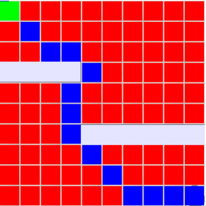
Fig 7.6: Output of Dijkstra algorithm​

There are some factors considered for the Dijkstra algorithm:

• There are two lists with the size of the map which are called parent and distance. Parent list stores the parent of the current node. and distance node basically stores of the cost distance value from the goal.
• For every iteration, it basically finds the distance for all the neighboring nodes and it stores it in the distance list, and also stores its parent nodes. This is done until the goal state is reached.
• After the iteration completes, we backtrack the start from the goal, based on the parent list.
• Here the red square in the image means that the algorithm is run throughout the map and each and every node is considered.
• The blue square is the backtracking of the algorithm, which basically shows the shortest path.
• The green square is the goal point. This is enabled when the iterations are completed.

7.2.2 Uniform Cost Search (UCS)

Uniform Cost Search is just a variant of Djikstra. Dijkstra algorithm searches for shortest paths from the root to every other node in a graph, whereas UCS searches for shortest paths in terms of cost to a goal node. The uniform Cost Search algorithm is the algorithm where starting state we will visit the adjacent state and will choose the least costly state then we will choose the next least costly state from all non visited and adjacent states of the visited states, in this way we will try to reach the goal state, even if we reach the goal state we will continue searching for other possible paths. We will keep a priority queue which will give the least costly next state from all the adjacent states of visited states. A weighted graph uses numbers to represent the cost of taking each path or course of action.

7.2.2.1 Terminology and Pseudocode of Uniform Cost Search:

Pseudocode of UCS algorithm:

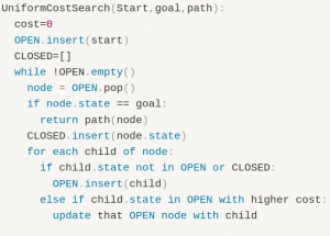
Fig 7.7: Psuedocode for the UCS algorithm​

The terminology used in the Pseudocode:

• Here OPEN and CLOSED are priority queues. Priority queues are abstract data structures where each data/value in the queue has a certain priority.
• In priority queues, .pop() is used to remove the last element of the list. .insert(location, value) is used to insert the value in the specified location.
• Here the cost is initially considered as zero. Every time we reach the child, the cost is added based on edge value.

7.2.2.2 Implementation of Uniform Cost Search in copeliasim:

The following image shows the output of the uniform cost search algorithm performed in the environment.

Fig 7.8: Output of Uniform Cost search algorithm

There are some factors considered for the uniform cost search algorithm:

• Here we have an open and closed list. The closed list includes all the nodes, which have already been visited. The open list includes all the nodes, which have the probability of going towards the goal. It also has the distance from the goal.
• For every iteration, the open list stores the neighboring nodes and also stores the distance cost from the current node.
• Here the red square in the image means that the algorithm is run throughout the map and each and every node is considered.
• The blue square is the backtracking of the algorithm, which basically shows the shortest path.
• The green square is the goal point. This is enabled when the iterations are completed.

7.2.3 A-star Search (A*)

A* Search is a searching algorithm that is used to find the shortest path between an initial and a final point. It was initially designed as a graph traversal problem, to help build a robot that can find its own course. It still remains a widely popular algorithm for graph traversal.

It searches for shorter paths first, thus making it an optimal and complete algorithm. An optimal algorithm will find the least cost outcome for a problem, while a complete algorithm finds all the possible outcomes of a problem.

A* is so powerful because of the use of weighted graphs in its implementation. A weighted graph uses numbers to represent the cost of taking each path or course of action. This means that the algorithms can take the path with the least cost, and find the best route in terms of distance and time.

A* algorithm has 3 parameters:

• Cost (g):  the cost of moving from the initial cell to the current cell. Basically, it is the sum of all the cells that have been visited since leaving the first cell.
• Heuristic (h): it is the estimated cost of moving from the current cell to the final cell. The actual cost cannot be calculated until the final cell is reached. Hence, h is the estimated cost. Here the heuristic used is the manhattan distance. Manhattan distance is the between two points measured along axes at right angles. In a plane with p₁ at (x₁, y₁) and p₂ at (x₂, y₂), it is |x₁ – x₂| + |y₁ – y₂|.
• Total cost (f): it is the sum of g and h. So, f= h + g

The way that the algorithm makes its decisions is by taking the f-value into account. The algorithm selects the smallest f-valued cell and moves to that cell. This process continues until the algorithm reaches its goal cell.

The algorithm is explained using an example in the video below:

7.2.3.1 Terminology and Pseudocode of A*

Pseudocode of A* algorithm:

Fig 7.9: Pseudocode for the A-Star algorithm​

The terminology used in the Pseudocode:

• Here OPEN and CLOSED are priority queues. Priority Queues are abstract data structures where each data/value in the queue has a certain priority.
• In priority queues, .pop() is used to remove the last element of the list. .insert(location, value) is used to insert the value in the specified location.
• Here the cost is initially considered as zero. Every time we reach the child state is reached, the cost is added based on edge value.

7.2.3.2 Implementation of A* in copeliasim:

The following image shows the output of the A* algorithm performed in the environment.

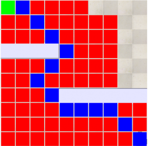
Fig 7.10: Output of A* algorithm

There are some factors considered for the A*  algorithm:

• All the factors are similar to UCS, except it has an additional heuristic. Here the heuristic method is the manhattan distance explained above.
• One thing which is different from other grid planning techniques is that the A* doesn’t have to check all the nodes in the map, because of the heuristic. Heuristic enables to check the nodes which are actually closer to the goal.

7.2.4 Comparison of various Grid Methods

When I compared the three grid-based motion planning algorithms, the most efficient was A*, when compared to Dijkstra and Uniform cost search. The heuristic in the A* made the grid-based motion planning efficient because of checking only the nodes, which are closer to the goal. Dijkstra is comparatively slow compared to A*, but it was actually faster than uniform cost search because we had a separate list for distance and parent, which was easily accessible. In uniform cost search, the ability to determine the distance cost and checking the neighbors, and also tracking the nodes from the start in a single list, basically occupies huge storage and slows the process.

7.3 Sampling Methods

Sampling-based algorithms represent the configuration space with a roadmap of sampled configurations. it creates possible paths by randomly adding points to a tree until some solution is found or time expires. As the probability to find a path approaches one when times go to infinity, sampling-based path planners are probabilistic complete. Configuration space is a collision-free space where the robot is able to move inside the path considering the robot’s dimensions. The following image is of the configuration space for our simulation. The white represents the collision-free space. Here the obstacle thickness is more than the actual size because the robot dimension is also added so that it doesn’t collide, irrespective of robot orientation.

Fig 7.11: Configuration space for the sampling method in copeliasim

They are popular for the following reasons:

• They often produce paths quickly for high-dimensional problems that are not too-maze, and given enough time can eventually solve problems of arbitrary complexity.
• By “high-dimensional” we mean that sampling-based planners can routinely solve problems in spaces of approximately 10D, and with tuning, we can also find feasible paths in dozens or even hundreds of dimensions.

7.3.1 Probabilistic Road Map Planner (PRM)

A probabilistic Road map planner is a sampling algorithm, which solves the problem of determining a path between a starting configuration of the robot and a goal configuration while avoiding collisions. It is used mainly to solve complex motion planning problems in high-dimensional configuration space.

A probabilistic roadmap planner consists of two phases:

• Construction Phase: A graph is built, which can be made in the environment. First, a random configuration is created. Then, it is connected to some neighbors, typically either the k nearest neighbors or all neighbors less than some predetermined distance. Configurations and connections are added to the graph until the roadmap is complete enough to connect the start and goal.
• Query Phase: the start and goal configurations are connected to the graph, and the path is obtained by the A* query.

7.3.1.1 Terminology and Pseudocode of PRM Planner

Pseudocode of PRM Planner:

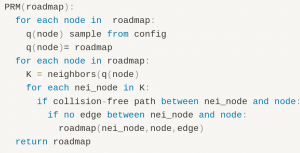
Fig 7.12: Psuedocode for the PRM Planner​

The terminology used in the Pseudocode:

• the roadmap contains the map with obstacles. Nodes are generated in the roadmap by sampling in the configuration space
• neighbors() function helps to find all the neighboring nodes from the current node (Inside a particular radius), which is created by sampling.
• roadmap(node1, node2,edge) creates a edge between two nodes added in the arguments.

7.3.1.2 Implementation of PRM Planner in copeliasim:

The following image shows the output of the PRM Planner performed in the environment.

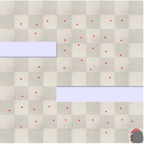
Fig 7.13: Randomly generating points inside the configuration space

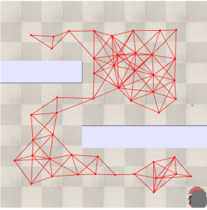
Fig 7.14: Joining these points to complete the construction phase of PRM

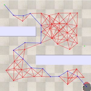
Fig 7.15: A* implementation in the query phase of the PRM Planner

There are some factors considered for the PRM Planner:

• We randomly generate points inside the configuration space and these points are joined with their neighboring points with a particular radius. This is basically the construction phase in PRM Planner.
• For the query phase, the construction phase output is considered as a graph where the distance is the weights in the graph, which basically needs an algorithm for determining the fastest route. Here we are using the A* algorithm for the fastest route.

7.3.2 Rapidly Exploring Random Tree (RRT)

RRT algorithm is a prepossess where points are randomly generated and connected to the closest available node. Each time a vertex is created, a check must be made that the vertex lies outside of an obstacle. Furthermore, chaining the vertex to its closest neighbor must also avoid obstacles. The algorithm ends when a node is generated within the goal region, or a limit is hit.

7.3.2.1 Terminology and Pseudocode of RRT

Pseudocode of RRT algorithm:

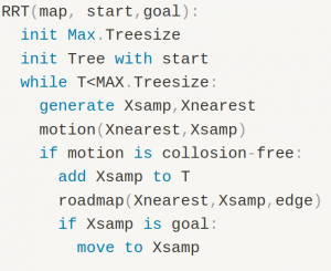
Fig 7.16: Psuedocode for the RRT Planner

7.3.2.2 Implementation of RRT in copeliasim:

The following image shows the output of the RRT algorithm performed in the environment

Fig 7.17: RRT Implementation in copeliasim

There are some factors considered for the RRT:

• In this algorithm, we use a finite number of iterations. As the iteration number increases, we have more ways to move from start to goal.
• The Tree generated should be inside the obstacle-free space of the configuration space we created.
• We also have a list that basically holds all the nodes which are part of the tree. This is created because in order to check the closest node of the tree to the sampled random node created.

7.3.3 Rapidly exploring Random Tree-Star (RRT *)

RRT* is an optimized version of RRT. When the number of nodes approaches infinity, the RRT* algorithm will deliver the shortest possible path to the goal. While realistically unfeasible, this statement suggests that the algorithm does work to develop the shortest path. It has two elements that differentiate it from RRT:

• First, RRT* records the distance each vertex has traveled relative to its parent vertex. This is referred to as the cost()of the vertex. After the closest node is found in the graph, a neighborhood of vertices in a fixed radius from the new node is examined. If a node with a cheaper cost than the proximal node is found, the cheaper node replaces the proximal node
• The second difference RRT* adds is the rewiring of the tree. After a vertex has been connected to the cheapest neighbor, the neighbors are again examined. Neighbors are checked if being rewired to the newly added vertex will make their cost decrease. If the cost does indeed decrease, the neighbor is rewired to the newly added vertex.

7.3.3.1 Terminology and Pseudocode of RRT*

Pseudocode of RRT* Planner:

Fig 7.18: Psuedocode for the RRT* Planner

7.3.3.2 Implementation of RRT* in copeliasim:

The following image shows the output of the RRT* algorithm performed in the environment

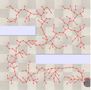
Fig 7.19: RRT* implementation in copeliasim

There are some factors considered for the RRT*:

• All the factors are similar to RRT, except it has a cost function in a particular radius.
• This cost function used here basically determines all the nodes of the tree, which is within a particular radius of the random node created. This function basically finds the shortest way from these tree points to the random point generated.

7.3.4 Comparison of Various Sampling Methods

RRT and RRT* are very efficient compared to PRM planner because the PRM planner requires creating a graph and then we use A* for determining the shortest path, which is time-consuming and occupies huge storage. RRT and RRT* are motion planning algorithms that require a single query for the output. PRM planner requires multiple query based on the complexity of the problem.

References

[1] LaValle, S. M. (2014). Planning algorithms. Cambridge University Press.