
3 Inverse Kinematics
Akshit Lunia
Chapter 3 Inverse Kinematics
3.1. General Inverse Kinematics Problem
Example – 2-Link Planar Manipulator
3.2. Analytical Approach
3.2.1. Geometrical Approach
3.2.2. Algebraic Approach
Example – 2-Link Planar Manipulator
3.3. Iterative Numerical Approach
3.3.1. Newton-Raphson Method
3.4. Kinematic Decoupling
Example – 6 DoF Robot Manipulator
3.4.1. Inverse Position
Example – 6 DoF Robot Manipulator (Continued)
3.4.2. Inverse Orientation
3.4.2.1. Euler Angle Parameterization
Example – 6 DoF Robot Manipulator (Continued)
3.5. Summary
Practice Questions
Simulation and Animation
References
Introduction to Inverse Kinematics
Inverse kinematics (IK) is a method of solving the joint variables when the end-effector position and orientation (relative to the base frame) of a serial chain manipulator and all the geometric link parameters are known.
In this chapter, we begin by understanding the general IK problem. After which we observe various methods used to solve IK, we explore the analytical approaches to solve the inverse position problem; specifically, we will investigate the geometric and algebraic techniques. We will also discuss the numerical iterative method to solve a higher degree-of-freedom (DoF) inverse kinematic problem. Further on, we describe the principle of kinematic decoupling and how it helps simplify our solution by splitting a higher DoF robotic manipulator into simplified inverse orientation and inverse position problems. To solve the inverse orientation problem, we use the Euler angle parameterization. Finally, we will conclude the chapter with some coding and simulation.
3.1. General Inverse Kinematics Problem
The general problem of IK is to find a solution or multiple solutions when a 4 × 4 homogeneous transformation matrix is given:
| [latex]H_n^0= \left[\begin{matrix}R_n^0&o_n^0\\0&1\\\end{matrix}\right][/latex] ∈ SE (3) | 3.1 |
As we know, the above homogenous transformation matrix provides us with the end-effector orientation (3 × 3 matrix) and position (a 3×1 vector providing the coordinates of the end-effector origin) with respect to the base frame.
We know from the forward kinematics chapter (Chapter 2 ) that for an [latex]n[/latex] – DoF manipulator,
| [latex]H = T_n^0 = A_1\left(q_1\right).\ \ .\ \ .\ A_n\left(q_n\right)[/latex] | 3.2 |
By using this relation, we can find the solution for joint variables [latex]q_1, q_2,q_3, . . . , q_n[/latex]
Example: To better understand the inverse kinematic problem, let us consider a 2 – link planar manipulator
Assumptions:
- [latex]a_1 > a_2[/latex]
- revolute joints can revolve complete 180°
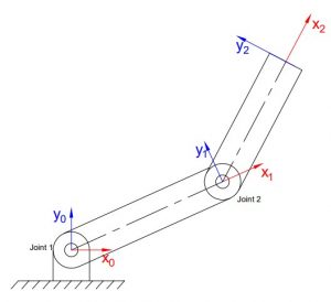
Fig 3.1. (a)

Fig 3.1. (b)
Fig 3.1. Revolute-Revolute (RR) planar robot manipulator where (a) Elbow-down configuration, (b) Elbow-up configuration
Denavit-Hartenberg (DH) Table:
| Link | [latex]a_i[/latex] | [latex]\alpha_i[/latex] | [latex]d_i[/latex] | [latex]\theta_i[/latex] |
| 1 | [latex]a_1[/latex] | 0 | 0 | [latex]ϴ1[/latex] |
| 2 | [latex]a_2[/latex] | 0 | 0 | [latex]ϴ2[/latex] |
From the DH Table using Forward Kinematics, we get
| [latex]H = T_2^0 = \left[\begin{matrix}c_{12}&{-s}_{12}&0&a_1c_1\ +\ {a_2c}_{12}\\s_{12}&c_{12}&0&a_1s_1\ +\ {a_2s}_{12}\\0&0&1&0\\0&0&0&1\\\end{matrix}\right][/latex] | 3.3 |
For simplification:
[latex]c_1[/latex] = cos([latex]ϴ_1[/latex])
[latex]s_1[/latex] = sin ([latex]ϴ_2[/latex])
[latex]c_{12}[/latex] = cos([latex]ϴ_1+ϴ_2[/latex])
[latex]s_{12}[/latex] = sin([latex]ϴ_1+ϴ_2[/latex])
We know,
| [latex]\left[\begin{matrix}x_2^0\\y_2^0\\\end{matrix}\right] = \left[\begin{matrix}a_1c_1\ +\ {a_2c}_{12}\\a_1s_1\ +\ {a_2s}_{12}\\\end{matrix}\right][/latex] | 3.4 |
Known values:
[latex](x_2,y_2)[/latex] = end-effector coordinates in cartesian space
[latex]x_2^0[/latex] = end – effector coordinate with respect to the base frame
[latex]y_2^0[/latex] = end – effector coordinate with respect to the base frame
[latex]a_1[/latex] = length of link 1
[latex]a_2[/latex] = length of link 2
Unknown variables:
[latex]ϴ_1[/latex] = angle of link 1 with the horizontal axis
[latex]ϴ_2[/latex] = angle of link 2 with the horizontal axis
For a given end-effector position ([latex]x, y[/latex]), we can have no solution (when the end-effector position lies outside the workspace area), one unique solution, or two solutions. Figure (no. to be assigned) shows that two solutions (elbow-up & elbow-down) correspond to the different joint configurations that give the same end-effector position.
To find an explicit solution for joint angles, we use the Atan2 or Arctan2 function. It provides an explicit value of[latex]ϴ[/latex] such that [latex]-π < ϴ < π[/latex].
Using the triangle made by the two links,
- For elbow-down configuration:
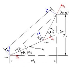
Fig 3.2. Geometric Illustration for the elbow down configuration
| [latex]Ф_3 = arctan\left(\frac{y_2^0}{x_2^0}\right)[/latex] | 3.5 |
| [latex]r = \sqrt{{(x_2^0)}^2\ +\ {(y_2^0)}^2}[/latex] | 3.6 |
Using law of cosine:
| [latex](a_2)^2 = (a_1)^2 + r^2 - 2a_1rcos(Ф_1)[/latex] | 3.7 |
| [latex]\therefore Ф_1 = arccos\left(\frac{\ {(a_1)}^2\ +\ \ r^2\ -\ {(a_2)}^2}{2a_1r}\right)[/latex] | 3.8 |
| [latex]\therefore[/latex][latex]ϴ_1 = Ф_3 - Ф_1[/latex] | 3.9 |
By substituting the corresponding values of [latex]Ф_3[/latex] we can solve for [latex]ϴ_2[/latex] we can solve for [latex]ϴ_1[/latex].
Similarly,
Using law of cosine:
| [latex]r_2 = (a_1)^2 + (a_2)^2 - 2 a_1a_2cos(Ф_2)[/latex] | 3.10 |
| [latex]\therefore Ф_2 = arccos\left(\frac{\ {(a_1)}^2\ +\ \ {(a_2)}^2\ -\ \ r_2}{2a_1a_2}\right)[/latex] | 3.11 |
| [latex]\therefore[/latex][latex]ϴ_2 = π – Ф_2[/latex] | 3.12 |
By substituting the corresponding values of [latex]Ф_2[/latex], we can solve for [latex]ϴ_2[/latex].
2. For elbow-up configuration:
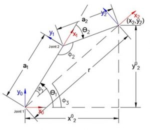
Fig 3.3. Geometric Illustration for the elbow-up configuration
Similar to how we solved for the elbow-down configuration, we substitute the values found using trigonometry into the following equations:
| [latex]ϴ_1 = Ф_3 + Ф_1[/latex] | 3.13 |
| [latex]ϴ_2 = Ф_2 – π[/latex] | 3.14 |
(Note: [latex]ϴ_2+Ф_2 = π[/latex] according to the diagram, but since the angle is measured in the clockwise direction, we take it as [latex]-ϴ_2[/latex]. Hence, [latex]- ϴ_2+Ф_2 = π[/latex], i.e. [latex]ϴ_2 = Ф_2 – π[/latex])
This method of finding the joint values for the desired end-effector position is known as inverse kinematics solution. In particular, this method of finding the joint equations is known as the geometric approach and we will be further exploring this in section 3.3.1 and section 3.4.1.
As the degree-of-freedom (DoF) in the manipulator increases, the complexity of the problem increases, and we can have more than two solutions (possibly infinite). With an increasing number of DoF, we also need to solve for redundancy and singularities.
3.2. Analytical Approach
In the general problem of IK (Section 3.1), we understood that a 4 × 4 homogeneous transformation matrix is used to define the position and orientation of the end-effector of a robot. We know from the forward kinematics chapter (Chapter 2) that the position of end-effector ([latex]{X}[/latex]) is a function of joint variables([latex]q_i[/latex]):
[latex]\\{X}=f\left({q}_{i}\right)[/latex]
Similarly,
| [latex]{q}_{i}=f^{-1}\left({X}\right)[/latex] | 3.15 |
Solving for IK requires us to solve for the joint variables when the end-effector’s position is provided (3.15). To solve for joint variables, there are two distinct methods:
(i) Analytical Method
Geometric Method
Algebraic Method
(ii) Numerical Iterative
The analytical method solves Equation (3.15) analytically to produce all possible solutions for a given inverse kinematic problem. Depending on the DoF of a robot manipulator, the number of solutions varies. For manipulators with a fewer DoF than that of the end-effector, there are possibilities of no solution; in cases where there are too many degrees of freedom, there can be infinite solutions. The analytical method is further divided into two methods called geometric and algebraic methods, based on how we find the equations. As we move ahead to solve the IK problem for different robot manipulators using the analytical method, we observe that as the number of joints increases, the complexity of solving inverse kinematic using the analytical method becomes more unfeasible.
3.2.1. Geometrical Approach
The geometrical approach to solving IK decomposes the geometry of the robot manipulator, consisting of linkage and joints, into multiple planar problems. Converting a 3D problem to several 2D problems is quite straightforward for certain configurations of robot manipulators but may require some level of intuition and experience. The equations found after solving each 2D problem are then used to solve for joint variables using algebraic manipulation. Observe the example solved in section 3.1, it uses the geometry of the manipulator to form a trigonometric relationship between the desired end-effector position and joint values. We will further use this method to solve a 6-DoF robot manipulator in section 3.4.1, where we convert a 3D manipulator geometry into multiple planar geometries.
3.2.2. Algebraic Approach
The algebraic approach to solving IK uses the forward kinematics solution that we already know for a robot manipulator and uses the homogeneous transformation matrix to find the necessary joint equations and solves them algebraically. There is no systematic way to solve for multiple solutions like you do in the geometrical approach. It does not include observing the geometrical aspects of the robot manipulator to find the equations.
When comparing with the geometric approach, the algebraic approach relies on the solution of forward kinematics whereas the geometrical approach only relies on the geometry of the robot manipulator (obviously both require the end-effector position in the form of a 4×4 homogeneous transformation matrix).
Example: Let us take the same RR 2-link planar robot manipulator.
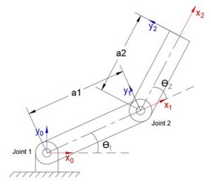
Fig 3.4. RR 2-link planar robot manipulator
As explained, the above algebraic approach takes the forward kinematics of the robot manipulator and extracts the joint equations from the forward kinematic solution. Let’s begin by first writing down the DH table.
| Link | [latex]a_i[/latex] | [latex]\alpha_i[/latex] | [latex]d_i[/latex] | [latex]\theta_i[/latex] |
| 1 | [latex]a_1[/latex] | 0 | 0 | [latex]\theta_1[/latex] |
| 2 | [latex]a_2[/latex] | 0 | 0 | [latex]\theta_2[/latex] |
Now using the DH table, we can find the [latex]A_{i\ }[/latex] matrices for links 1 and 2. using the following formula:
| [latex]A_{i\ }=\ \left[\begin{matrix}c_{\theta_i}&-s_{\theta_i}c_{\alpha_i}&s_{\theta_i}s_{\alpha_i}&a_ic_{\theta_i}\\s_{\theta_i}&c_{\theta_i}c_{\alpha_i}&-c_{\theta_i}s_{\alpha_i}&a_is_{\theta_i}\\0&s_{\alpha_i}&c_{\alpha_i}&d_i\\0&0&0&1\\\end{matrix}\right][/latex] | 3.16 |
Using Equation 3.16, we have the following:
[latex]\therefore A_1=\ \left[\begin{matrix}c_{\theta_1}&-s_{\theta_1}c_{\alpha_1}&s_{\theta_1}s_{\alpha_1}&a_1c_{\theta_1}\\s_{\theta_1}&c_{\theta_1}c_{\alpha_1}&-c_{\theta_1}s_{\alpha_1}&a_1s_{\theta_1}\\0&s_{\alpha_1}&c_{\alpha_1}&d_1\\0&0&0&1\\\end{matrix}\right]\ =\ \left[\begin{matrix}c_{\theta_1}&-s_{\theta_1}&0&a_1c_{\theta_1}\\s_{\theta_1}&c_{\theta_1}&0&a_1s_{\theta_1}\\0&0&1&d_1\\0&0&0&1\\\end{matrix}\right][/latex]
[latex]\therefore\ A_{2\ }=\ \left[\begin{matrix}c_{\theta_2}&-s_{\theta_2}c_{\alpha_2}&s_{\theta_2}s_{\alpha_2}&a_2c_{\theta_2}\\s_{\theta_2}&c_{\theta_2}c_{\alpha_2}&-c_{\theta_2}s_{\alpha_2}&a_2s_{\theta_2}\\0&s_{\alpha_2}&c_{\alpha_2}&d_2\\0&0&0&1\\\end{matrix}\right]=\ \left[\begin{matrix}c_{\theta_2}&-s_{\theta_2}&0&a_2c_{\theta_2}\\s_{\theta_2}&c_{\theta_2}&0&a_2s_{\theta_2}\\0&0&1&d_2\\0&0&0&1\\\end{matrix}\right][/latex]
Using the [latex]A_{i\ }[/latex] matrices, we find the homogeneous transformation matrix for the robot manipulator:
[latex]H_2^0\ =\ A_1A_2[/latex]
| [latex]{\therefore}H_2^0 = \left[\begin{matrix}c_{12}&{-s}_{12}&0&a_1c_1\ +\ {a_2c}_{12}\\s_{12}&c_{12}&0&a_1s_1\ +\ {a_2s}_{12}\\0&0&1&0\\0&0&0&1\\\end{matrix}\right][/latex] | 3.17 |
The last column of the homogenous matrix [latex]H_2^0[/latex] provides the position of the end-effector in the frame {0}. Therefore,
| [latex]x_2^0\ =\ a_1c_1\ +\ {a_2c}_{12}[/latex] | 3.18 |
| [latex]y_2^0\ =a_1s_1\ +\ {a_2s}_{12}[/latex] | 3.19 |
| [latex]z_2^0\ =\ 0[/latex] | 3.20 |
By squaring and adding equations 3.18 and 3.19, we get,
[latex]{(x_2^0)}^2+{(y_2^0)}^2\ ={(a_1)}^2+{(a_2)}^2+{2a_1a}_2c_2[/latex]
[latex]\therefore\theta_2=\ \cos^{-1}\left(\frac{{(x_2^0)}^2+{(y_2^0)}^2-{(a_2)}^2-{(a_2)}^2}{{2a_1a}_2}\right)[/latex]
According to Equation 3.19, it follows that
[latex]y_2^0\ =a_1sin\theta_1\ +\ a_2(c_2sin\theta_1+s_2cos\theta_1)=\ (a_1+a_2c_2)sin\theta_1+a_2s_2cos\theta_1[/latex]
The above equation is in the form [latex]acos\theta+bsin\theta=c[/latex] for which,
[latex]\theta\ =\ \tan^{-1}\left(\frac{c}{\pm\sqrt{a^2+b^2-c^2}}\right)-\tan^{-1}\left(\frac{a}{b}\right)[/latex]
[latex]\therefore\theta_{1\ }=\tan^{-1}\left(\frac{y_2^0}{\sqrt{{(a_1+a_2c_2)}^2+{{(a}_2s_2)}^2-{{(y}_2^0)}^2}}\right)-\tan^{-1}\left(\frac{a_2s_2}{(a_1+a_2c_2)}\right)[/latex]
[latex]=\ \tan^{-1}\left(\frac{y_2^0}{\sqrt{{(a_1)}^2+{(a_2)}^2+{2a_1a}_2c_2-{{(y}_2^0)}^2}}\right)-\tan^{-1}\left(\frac{a_2s_2}{(a_1+a_2c_2)}\right)[/latex]
[latex]=\tan^{-1}\left(\frac{y_2^0}{\sqrt{{(x_2^0)}^2+{(y_2^0)}^2-{{(y}_2^0)}^2}}\right)-\tan^{-1}\left(\frac{a_2s_2}{(a_1+a_2c_2)}\right)[/latex]
[latex]=\ \tan^{-1}\left(\frac{y_2^0}{x_2^0}\right)-\tan^{-1}\left(\frac{a_2s_2}{(a_1+a_2c_2)}\right)[/latex]
Using the algebraic approach, we found the values of [latex]\theta_1[/latex] and [latex]\theta_2[/latex].
3.3. Iterative Numerical Approach
Numerical solutions, unlike analytical solutions, are robot independent and may thus be used for any kinematic structure. Only when the polynomial equations have four or fewer degrees may analytical solutions be found. The analytical solution fails to provide a solution if the degree of the polynomial is higher. As a result, even if the DOF is less than or equal to 6, many manipulator geometries are not solvable. In general, higher numbers of non-zero geometric parameters correspond to a higher degree of the polynomials, which makes the analytical approach unfeasible. We utilize a numerical approach to solve such manipulator geometries.
There are different ways to solve IK using the numerical method. We will be using the Newton-Raphson method since it is one of the faster ways to find solutions for nonlinear equations.
3.3.1. Newton-Raphson Method
We know from the forward kinematics chapter that a robot manipulator’s end-effector position(x) can be defined as a differentiable function of joint variables. Let us assume that we are solving for a robot manipulator with only revolute joints. Therefore,
[latex]x\ =\ f(\theta)[/latex]
Let [latex]x_d[/latex] and [latex]\theta_d[/latex] be the desired end-effector position and joint values to reach the desired joint variable. Thus the inverse kinematic can be defined as:
[latex]x_d\ – f(\theta_d) = 0[/latex]
This equation represents the Newton-Raphson method, and the goal is to find [latex]\theta_d[/latex].
According to the Newton-Raphson method, we can solve nonlinear polynomials by making an initial guess and using that to converge towards a root/solution (it doesn’t necessarily solve for the closest root). Let’s look at a polynomial curve for which we want to find a solution:
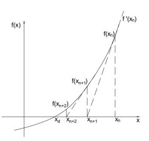
Fig 3.5. Solution illustration for the numerical approach
The Newton-Raphson method begins with the selection of an initial guess ([latex]x_n[/latex]), which is closer to the solution [latex]x_d[/latex], from where we find the slope [latex]f^\prime\left(x_n\right)[/latex]. When extended we can see that the slope intersects at the x-axis giving us a new point ([latex]x_{n+1}[/latex]). We then evaluate the slope [latex]f^\prime\left(x_{n+1}\right)[/latex] at point [latex]x_{n+1}[/latex]. The slope then intersects at a new point [latex]x_{n+2}[/latex] and the process repeats converging towards the solution [latex]x_d[/latex].
We can derive the formula for a better approximation ([latex]x_{n+1}[/latex]) using Fig 3.5. The tangent [latex]f^\prime\left(x_n\right)[/latex] can be defined as
[latex]y=f^\prime\left(x_n\right)\left(x-x_n\right)+f\left(x_n\right)[/latex]
The x-intercept ([latex]y=0[/latex]) of the tangent [latex]f^\prime\left(x_n\right)[/latex] will give us the point [latex]x_{n+1}[/latex]. Therefore,
[latex]0=f\left(x_n\right)+f^\prime\left(x_n\right)\left(x_{n+1}-x_n\right)[/latex][latex]\therefore\ x_{n+1}=x_n-\left(\frac{df\left(x\right)}{dx}\right)^{-1}f\left(x_n\right)[/latex]
Since we are considering a vector in IK, we have
[latex]\vec{x}=\left[\begin{matrix}\theta_1\\\vdots\\\theta_n\\\end{matrix}\right][/latex]
| [latex]{\therefore\ x}_{n+1}=x_n-\left(\frac{\partial F\left(x\right)}{\partial x}\right)^{-1}|_{x_n}F\left(x_n\right)[/latex] | 3.21 |
Where, [latex]\frac{\partial F\left(x\right)}{\partial x}[/latex] is the Jacobian matrix.
We iterate till we reach the end-effector position. Sometimes, the function curve is such that we don’t reach the end-effector position even after many iterations (the approximation doesn’t converge towards the solution). In such cases, we take a new initial guess ([latex]x_n[/latex]) and start new iterations.
3.4. Kinematic Decoupling
The previous examples refer to a very basic inverse kinematic problem of a 2D and 3D robotic manipulator. But as we increase the DoF the complexity increases significantly.
Certain manipulators can be solved by simplifying or breaking the problem into two smaller problems: inverse position and inverse orientation when there is a spherical wrist present in the robotic manipulator. A spherical wrist such as the Stanford manipulator has 3 revolute joints with the actuation axis that intersect at a common point. When we observe a 6-DOF robotic manipulator with a spherical wrist (figure 3.6 ) we can observe that the position of the wrist is affected by the first three joints of the manipulator, i.e., even when we actuate the fourth, fifth, or sixth joint the position of the wrist doesn’t change.
The overall transformation matrix can then be decomposed to a translation and rotation matrix, each having three unknown parameters:
| [latex]T_6^0 = \left[\begin{matrix}R_6^0&o_6^0\\0&1\\\end{matrix}\right] = O_6^0R_6^0 = \left[\begin{matrix}I&o_6^0\\0&1\\\end{matrix}\right]\left[\begin{matrix}R_6^0&0\\0&1\\\end{matrix}\right][/latex] | 3.22 |
Where,
[latex]O_6^0[/latex] indicates the position of the end-effector with respect to the base frame
[latex]R_6^0[/latex] indicates the orientation of the end-effector with respect to the base frame
Example: Let’s look at a 6-DOF robot manipulator with a spherical wrist:
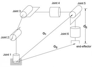
Figure 3.6. 6-DOF Robot manipulator model
DH Table:
| Link | ai | [latex]\alpha_i[/latex] | di | [latex]\theta_i[/latex] |
| 1 | 0 | 90 | d1 | [latex]\theta_1[/latex] |
| 2 | a2 | 0 | 0 | [latex]\theta_2[/latex] |
| 3 | a3 | 0 | 0 | [latex]\theta_3[/latex] |
| 4 | 0 | -90 | 0 | [latex]\theta_4[/latex] |
| 5 | 0 | 0 | 0 | [latex]\theta_5[/latex] |
| 6 | 0 | 0 | d6 | [latex]\theta_6[/latex] |
We are provided with the forward kinematics such that,
[latex]o = \left[\begin{matrix}o_x\\o_y\\o_z\\\end{matrix}\right][/latex] and [latex]R = \left[\begin{matrix}r_{11}&r_{12}&r_{13}\\r_{21}&r_{22}&r_{23}\\r_{31}&r_{32}&r_{33}\\\end{matrix}\right][/latex]
Step 1 : Find the Wrist point [latex]o_c[/latex]
[latex]\left[\begin{matrix}x_c\\y_c\\z_c\\\end{matrix}\right] = \left[\begin{matrix}o_x\ -\ a_6r_{13}\\o_y-\ a_6r_{23}\\o_z-\ a_6r_{33}\\\end{matrix}\right][/latex]
Let us now look at how decoupling of the manipulator and solving its inverse position and orientation problem reduces the difficulty in finding a solution.
3.4.1. Inverse Position
We can use a geometric approach to solve for the most common kinematic arrangements to find the joint variables for the first three joints ([latex]q_1, q_2[/latex], and [latex]q_3[/latex]) corresponding to the wrist center point ([latex]o_c[/latex]).
With the increasing number of nonzero components in the DH table, the difficulty of using the geometric approach to solve the inverse kinematic problem increases, but for our example, with very few nonzero terms in the DH table, the geometric approach is suitable. The general idea of a geometric method is to solve for joint variables by projecting the geometry of the robot manipulator on the [latex]x_{i-1}[/latex] and [latex]y_{i-1}[/latex] plane and using trigonometry to solve.
Continuing with our solution:
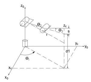
Fig 3.7. Geometric illustration of a 6-DOF robot model highlighting the first three joints [1]
Step 2: Finding joint 1 angle ([latex]ϴ_1[/latex])
Observing the first joint, we can see that joint one only affects the x and y coordinates of the wrist point. So, we can reduce the problem to a 2D planar problem.
| [latex]\therefore ϴ_1 = Atan2(x_c,\ y_c)[/latex] | 3.23 |
However, two solutions are possible here due to Atan2 function:
| [latex]\therefore ϴ_1 = π + Atan2(x_c,\ y_c)[/latex] | 3.24 |
Step 3: Finding joint 2 and joint 3 angles ([latex]ϴ_2[/latex] and [latex]ϴ_3[/latex] respectively)

Fig 3.8. Side view of the first three joints of the 6 DoF manipulator illustrated in Fig 3.6
Similar to joint 1, we can observe that the movement of joints 2 and 3 only takes place in the vertical plane. Hence, we can simplify the problem to a 2D planar problem.
This problem is like the 2-link planar manipulator in section 3.1.
Elbow–down configuration solution:
| [latex]Ф_3 = arctan\left(\frac{z_3^0-a_1}{x_3^0}\right)[/latex] | 3.25 |
| [latex]r = \sqrt{{(x_3^0)}^2\ +\ {(z_3^0-a_1)}^2}[/latex] | 3.26 |
Using law of cosine:
| [latex](a_3)^2 = (a_2)^2 + r^2 - 2a_2rcos(Ф_1)[/latex] | 3.27 |
| [latex]\therefore Ф_1 = arccos\left(\frac{\ {(a_2)}^2\ +\ \ r^2\ -\ {(a_3)}^2}{2a_2r}\right)[/latex] | 3.28 |
| [latex]\therefore ϴ_1 = Ф_3 - Ф_1[/latex] | 3.29 |
Similarly, using the law of cosine:
| [latex]r^2 = (a_2)^2 + (a_3)^2 - 2a_2a_3cos(Ф_2)[/latex] | 3.30 |
| [latex]\therefore Ф_2 = arccos\left(\frac{\ {(a_2)}^2\ +\ \ {(a_3)}^2\ -\ \ r^2}{2a_2a_3}\right)[/latex] | 3.31 |
| [latex]\therefore ϴ_2 = π – Ф_2[/latex] | 3.32 |
Elbow–up configuration solution:
We can follow the same procedure used previously to solve for this configuration and substitute in the following equations.
[latex]ϴ_1 = Ф_3 + Ф_1[/latex]
[latex]ϴ_2 = Ф_2 – π[/latex]
In this example, we assume no shoulder offset is present, hence only two possible inverse position solutions. There will be two additional inverse position solutions possible in the case of shoulder offsets like in the PUMA 6-DOF robotic arm below.
3.4.2. Inverse Orientation
The method used to solve the inverse position problem is called the geometric method. Using this method, we solved for the first three joint angles for a given wrist position. The inverse orientation problem is where we find the orientation of the wrist for a given end-effector orientation. To solve the inverse orientation problem, we take the help of Euler angles. Let us first take a brief look at Euler angles and how does it help us in solving the inverse orientation problem.
3.4.2.1. Euler Angle Parameterization:
Euler angles are a set of three angles, denoted as [latex]Ф, ϴ[/latex], and [latex]ψ[/latex], also known as the roll, pitch, and yaw. We can use these three angles to specify the orientation of a rotated frame about the base frame. There are various Euler angle transformations used (XYZ, ZYZ, ZYX, etc.). We will be using ZYZ Euler angles transformation.
As we have learned before, any orientation can be represented by a 3×3 rotation matrix. For example, let a rotation of angle [latex]Ф[/latex] about the z-axis, [latex]ϴ[/latex]about the y-axis, and [latex]ψ[/latex] about the z-axis corresponding to the following rotation matrices:
[latex]R_z(Ф)= \begin{bmatrix} c_Ф & -s_Ф & 0 \\ s_Ф & c_Ф & 0 \\ 0 & 0 & 1 \end{bmatrix}[/latex],
[latex]R_y(ϴ)= \begin{bmatrix} c_ϴ & 0 & s_ϴ \\ 0 & 1 & 0 \\ -s_ϴ & 0 & c_ϴ \end{bmatrix}[/latex],
[latex]R_z(\psi)= \begin{bmatrix} c_\psi & -s_\psi & 0 \\ s_\psi & c_\psi & 0 \\ 0 & 0 & 1 \end{bmatrix}[/latex].
[latex]\therefore R_{zyz}=R_z(Ф)R_y(ϴ)R_z(ψ)[/latex]
= [latex]\begin{bmatrix} c_Ф & -s_Ф & 0 \\ s_Ф & c_Ф & 0 \\ 0 & 0 & 1 \end{bmatrix}\begin{bmatrix} c_ϴ & 0 & s_ϴ \\ 0 & 1 & 0 \\ -s_ϴ & 0 & c_ϴ \end{bmatrix}\begin{bmatrix} c_\psi & -s_\psi & 0 \\ s_\psi & c_\psi & 0 \\ 0 & 0 & 1 \end{bmatrix}[/latex]
| [latex]\therefore R_{zyz}= \begin{bmatrix} c_Фc_ϴc_ψ - s_Ф s_ψ & -c_Фc_ϴs_ψ - s_Ф c_ψ & c_Фs_ϴ \\ s_Фc_ϴc_ψ + c_Ф s_ψ & -s_Фc_ϴs_ψ + c_Ф c_ψ & s_Фs_ϴ \\ -s_ϴc_ψ & s_ϴs_ψ & c_ϴ \end{bmatrix}[/latex] | 3.33 |
This ZYZ rotation matrix is known as the ZYZ-Euler angle transformation. We consider two cases when using Euler angle transformation to solve inverse position problem:
Case I: Both [latex]r_{13}[/latex] and [latex]r_{23}[/latex] are not zero
If both [latex]r_{13}[/latex] and [latex]r_{23}[/latex] are not zero, we can deduce that [latex]s_ϴ \neq 0[/latex] and so both [latex]r_{31}[/latex] and [latex]r_{32}[/latex] are not zero, then [latex]r_{33}\ \neq\ \pm\ 1[/latex] and so [latex]r_{33}\ =\ c_ϴ[/latex].
Therefore,
| [latex]\therefore\theta=Atan2\left(r_{33},\sqrt{1\ -\ {{(r}_{33})}^2}\right)[/latex] | 3.34 |
Or
| [latex]\therefore\theta=Atan2\left(r_{33},-\sqrt{1\ -\ {{(r}_{33})}^2}\right)[/latex] | 3.35 |
If we choose the value of [latex]\theta[/latex] from equation (3.34), then
| [latex]\phi\ =\ Atan2\left(r_{13},r_{23}\right)[/latex] | 3.36 |
| [latex]\psi\ =\ Atan2\left(-r_{31},r_{32}\right)[/latex] | 3.37 |
If we choose the value of [latex]\theta[/latex] from equation (3.35), then
| [latex]\phi\ =\ Atan2\left(-r_{13},-r_{23}\right)[/latex] | 3.38 |
| [latex]\psi\ =\ Atan2\left(r_{31},-r_{32}\right)[/latex] | 3.39 |
Case II: R is an orthogonal matrix
If [latex]r_{13} = r_{23} = 0[/latex] and [latex]r_{31} = r_{32} = 0[/latex], then [latex]r_{33} = \pm\ 1[/latex]
If [latex]r_{33} = \ 1[/latex], then [latex]c_ϴ = 1[/latex], therefore [latex]\theta\ =\ 0[/latex]
In this case the equation (3.4.2.1) changes to:
[latex]\begin{bmatrix} c_Фc_ϴc_ψ - s_Ф s_ψ & -c_Фc_ϴs_ψ - s_Ф c_ψ & c_Фs_ϴ \\ s_Фc_ϴc_ψ + c_Ф s_ψ & -s_Фc_ϴs_ψ + c_Ф c_ψ & s_Фs_ϴ \\ -s_ϴc_ψ & s_ϴs_ψ & c_ϴ \end{bmatrix}[/latex] = [latex]\begin{bmatrix} c_{Ф+ψ} & -s_{Ф+ψ} & 0 \\ s_{Ф+ψ} & c_{Ф+ψ} & 0 \\ 0 & 0 & 1 \end{bmatrix}[/latex]
Thus,
[latex]\phi\ +\ \psi\ =\ Atan2\left(r_{11},-r_{12}\right)\ =\ \ Atan2\left(r_{11},r_{12}\right)[/latex]
Since, we are only able to determine the sum of the angles, there are infinitely many solutions.
If [latex]r_{33} = \ -\ 1[/latex], then [latex]c_ϴ = - 1[/latex], therefore [latex]\theta\ =\ \pi[/latex] in this case equation (3.2.2.1) changes to:
[latex]\begin{bmatrix} -c_{Ф+ψ} & -s_{Ф+ψ} & 0 \\ s_{Ф+ψ} & c_{Ф+ψ} & 0 \\ 0 & 0 & 1 \end{bmatrix}[/latex] = [latex]\begin{bmatrix} r_{11} & r_{12\ } & 0 \\ r_{21\ } & r_{22\ } & 0 \\ 0 & 0 & -1 \end{bmatrix}[/latex]
[latex]\phi\ -\ \psi\ =\ Atan2\left(-r_{11},-r_{12}\right)[/latex]
Similar to the case [latex]c_ϴ = 1[/latex], we have infinitely many solutions.
Now going back to solving the inverse orientation problem the of 6-DOF robot manipulator with a spherical wrist:
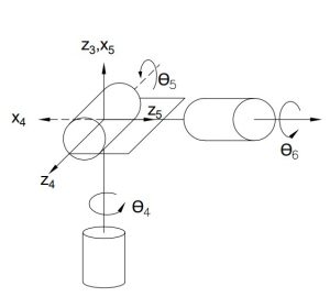
Fig 3.9. Spherical wrist in 6-DOF robot manipulator
Using the above explained Euler angle parameterization method, we select
[latex]\theta_4\ =\ Ф_,θ_5=ϴ,θ_6=ψ[/latex]
Using the DH parameter shown in the beginning of the problem, we solve for [latex]R_3^0[/latex] and [latex]R_6^3[/latex] :
[latex]R_3^0\ =\begin{bmatrix} c_1c_{23} & {-c}_1s_{23} & s_1\\ s_1c_{23} & -s_1s_{23} & -c_1 \\ s_{23}&c_{23}& 0 \end{bmatrix}[/latex]
[latex]R_6^3\ =\ \begin{bmatrix} c_4c_5c_6\ -\ s_4s_6&{-c}_4{c_5s}_{6\ }-\ s_4c_6&{c_4s}_5\\s_4c_5c_6\ +\ c_4s_6&{-s}_4{c_5s}_6+c_4c_6&{s_4s}_5\\{-s}_5c_6&s_5s_6&c_5 \end{bmatrix}[/latex]
We use the following equation to solve for the remaining three joint angles:
[latex]R_6^3\ =\ \left(R_3^0\right)^TR[/latex]
[latex]= \begin{bmatrix} c_1c_{23}&s_1c_{23}&s_{23}\\{-c}_1s_{23}&-s_1s_{23}&c_{23}\\s_1&-c_1&0 \end{bmatrix}[/latex][latex]\begin{bmatrix} r_{11}&r_{12}&r_{13}\\r_{21}&r_{22}&r_{23}\\r_{31}&r_{32}&r_{33} \end{bmatrix}[/latex]
= [latex]\begin{bmatrix} r_{31}s_{23}+s_1c_{23}r_{11}+c_{23}r_{21}s_1&r_{32}s_{23}+c_1c_{23}r_{12}+c_{23}r_{22}s_1&r_{33}s_{23}+c_1c_{23}r_{13}+c_{23}r_{23}s_1\\c_{23}r_{31}-c_1r_{11}s_{23}-r_{21}s_1s_{23}&c_{23}r_{32}-c_1r_{12}s23-r_{22}s_1s_{23}&c_{23}r_{33}-c_1r_{13}s_{23}-r_{23}s_1s_{23}\\\ r_{11}s_1\ -c_1r_{21}&r_{12}s_1\ -\ c_1r_{22}&r_{13}s_1\ -\ c_1r_{23} \end{bmatrix}[/latex]
To use Euler angle parameterization to find joint angles, we first need our rotation matrix to satisfy the Case I conditions.
| [latex]\therefore c_4s_5\ =\ r_{33}s_{23}+c_1c_{23}r_{13}+c_{23}r_{23}s_1[/latex] | 3.40 |
| [latex]\therefore s_4s_5\ =c_{23}r_{33}-c_1r_{13}s_{23}-r_{23}s_1s_{23}[/latex] | 3.41 |
| [latex]\therefore c_5\ =\ \ r_{13}s_1\ -\ c_1r_{23}[/latex] | 3.42 |
That is, if both of Equations (3.40) and (3.41) are not zero (since we know [latex]\theta_1[/latex], [latex]\theta_2[/latex], and [latex]\theta_3[/latex] as well as the desired rotation matrix) , we can use Euler angle parameterization to get value of [latex]\theta[/latex] using Equations (3.34) and (3.35).
| [latex]\theta_4\ =\ Atan2(r_{13}s_1\ -\ c_1r_{23},\ \pm\ \sqrt{1\ -\ \left(r_{13}s_1\ -\ c_1r_{23}\right)^2}[/latex] | 3.43 |
Corresponding to the positive or negative square root chosen we can further find [latex]\theta_5[/latex] and [latex]\theta_6[/latex] using Equations (3.36) – (3.39).
For positive square root:
| [latex]\theta_5=Atan2\left(r_{33}s_{23}+c_1c_{23}r_{13}+c_{23}r_{23}s_1,c_{23}r_{33}-c_1r_{13}s_{23}-r_{23}s_1s_{23}\right)[/latex] | 3.44 |
| [latex]\theta_6=Atan2\left(-\left(r_{11}s_1\ -c_1r_{21}\right),r_{12}s_1\ -\ c_1r_{22}\right)[/latex] | 3.45 |
For negative square root:
| [latex]\theta_5=Atan2\left(-\left(r_{33}s_{23}+c_1c_{23}r_{13}+c_{23}r_{23}s_1\right),-\left(c_{23}r_{33}-c_1r_{13}s_{23}-r_{23}s_1s_{23}\right)\right)[/latex] | 3.46 |
| [latex]\theta_6\ =\ Atan2\left(r_{11}s_1\ -c_1r_{21},-\left(r_{12}s_1\ -\ c_1r_{22}\right)\right)[/latex] | 3.47 |
If [latex]s_5=0[/latex], then the actuation axes z3 and z5 are collinear which is a singularity configuration, and only the sum of angles [latex]\theta_4[/latex] and [latex]\theta_6[/latex], i.e. [latex]\theta_4+\theta_6[/latex], is known. One way to solve such a problem is to arbitrarily choose a value for [latex]\theta_4[/latex] or [latex]\theta_6[/latex] and solve for the other angle.
3.5. Summary
This chapter presents an overview of how the fundamentals of IK can be applied to robot mechanisms. To control a robot manipulator to move it towards a specific end-effector position, it is necessary to solve the IK of that manipulator. IK can be explained as finding joint variables for a corresponding end-effector position. It uses equations that relate the joint variables to the end-effector position. There are multiple methods of finding these equations, some of which we discussed is the closed-form analytical approach and the numerical approach.
The analytical approach to solving IK is a straightforward method where we use the DH convention to find the joint equation in the case of the algebraic approach. In contrast, we evaluate the robot linkages and joint geometry using simple trigonometry in the geometric approach. But using an analytical approach becomes increasingly difficult as the DoF increases.
We then looked at how we can simplify the analytical solution of a robot manipulator with 6-DOF using kinematic decoupling. Kinematic decoupling is a helpful method of breaking down robot manipulators with spherical wrists into smaller inverse position and inverse orientation problems. We use numerical methods for higher DoF robots since analytical approaches don’t always provide a solution, and it becomes even more complex for robots with DOF>6.
The numerical method we discussed is the iterative method using Newton-Raphson, which converges an initial guess towards the desired solution. Newton-Raphson method has limitations because of its high dependence on the initial guess. This chapter doesn’t include a comprehensive overview of the numerical method but can be found in various texts that take an in-depth look.
Practice Questions
- Find the IK of the 3-link planar manipulator, in elbow down configuration, shown below using the algebraic approach, assuming link lengths [latex]a1[/latex],[latex]a2[/latex], and [latex]a3[/latex]. Let end-effector positions be ([latex]x_e,y_e[/latex]). (Assume an orientation: [latex]\gamma=\theta_1+\theta_2+\theta_3[/latex]) :

Answer:
[latex]x_3\ =\ x_e\ -a_3\cos^{-1}{\gamma}[/latex]
[latex]y_3\ =\ y_e\ -a_3\sin^{-1}{\gamma}[/latex]
[latex]\theta_1\ =\ \tan^{-1}{\frac{y_3}{x_3}}-\cos^{-1}{\frac{{(x_3)}^2+{(y_3)}^2+{(a_1)}^2-{(a_2)}^2}{2a_1\sqrt{{(x_3)}^2+{(y_3)}^2}}}[/latex]
[latex]\theta_2\ =\ \pi-\cos^{-1}{\frac{{(a_1)}^2+{(a_2)}^2-{(x_3)}^2-{(y_3)}^2}{2a_1a_2}}[/latex]
[latex]\theta_3\ =\ \gamma-\theta_1-\theta_2[/latex]
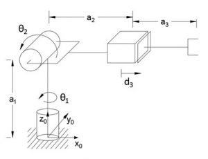
2. Find the inverse kinematic of the manipulator shown below using the geometric approach:
Answer:
[latex]\theta_1=arctan{\left(\frac{y_3^0}{x_3^0}\right)}[/latex]
[latex]\theta_2=arctan{\left(\frac{z_3^0-a_1}{\sqrt{\left(x_3^0\right)^2+\left(y_3^0\right)^2}}\right)}[/latex]
[latex]d_3=\sqrt{\left(z_3^0-a_1\right)^2+\left(x_3^0\right)^2+\left(y_3^0\right)^2}-a_2-a_3[/latex]
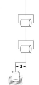
3. What will be the impact of shoulder offset on the solution of the first three joints (inverse position) of the 6-DOF robot manipulator discussed in the kinematic decoupling module (Section 3.4), you can refer to Figure 3.7? Find solutions for all four configurations. (Assume shoulder offset as ‘d’)
Answer:
There are four possible solutions for the inverse position of 6 – DoF robot manipulator with shoulder offset, they are:
(i) Left-arm elbow-up
(ii) Left-arm elbow-down
(iii) Right arm elbow-up
(iv) Right arm elbow-down
And the joint values are [1] :
[latex]\theta_1=Atan2\left(x_C,y_C\right)-Atan2\left(\sqrt{x_C^2+y_C^2-d^2},d\right)[/latex]
[latex]=Atan2\left(x_C,y_C\right)-Atan2\left(-\sqrt{x_C^2+y_C^2-d^2},-d\right)[/latex]
[latex]\theta_3=Atan2{\left(D,\pm\sqrt{1-D^2}\right)}[/latex]
Where, [latex]D=cos{\theta_3}=\frac{x_c^2+y_c^2-d^2+\left(z_c-d_1\right)^2-a_2^2-a_3^2}{2a_2a_3}[/latex]
[latex]\theta_2=Atan2{\left(\sqrt{x_c^2+y_c^2-d^2},z_c-d_1\right)}-Atan2{\left(a_2+a_3c_3,a_3s_3\right)}[/latex]
Simulation and Animation
Let’s try to use the methods we have learned in this chapter and try to find a solution to a 3-link planar manipulator and try simulating it in Coppeliasim software. You can check out the solution, simulation, and code here.
You can check the video of the simulation, here: recording_2021_12_13-21_28-11.
References
[1] Spong, M. W., Hutchinson, S., & Vidyasagar, M. (2020). Inverse Kinematics, ROBOT MODELING AND CONTROL SECOND EDITION (pp 141-162). Chichester, West Sussex, UK: John Wiley & Sons, Ltd.
[2] Lynch, K. (Kevin M.), & Park, F. C. (2017). Inverse Kinematics, MODERN ROBOTICS: MECHANICS, PLANNING, AND CONTROL (pp 219-244). Cambridge University Press.
[3] Waldron Kenneth and Schmiedeler, J. (2008). Kinematics. In O. Siciliano Bruno and Khatib (Ed.), Springer Handbook of Robotics (pp. 9–33). Springer Berlin Heidelberg. https://doi.org/10.1007/978-3-540-30301-5_2
[4] Craig, J. J., Prentice, P., & Hall, P. P. (2005). Inverse Manipulator Kinematics, Introduction to Robotics Mechanics and Control Third Edition (pp 101-134). Upper Saddle River, NJ: Pearson Education, Inc.
[5] Corke, P. (2017). Robot Arm Kinematics, Robotics, Vision and Control (Vol. 118) (pp 205-210). Springer International Publishing. https://doi.org/10.1007/978-3-319-54413-7
