
9 Motion and Force Control
Dennis Daly
Chapter Outlines
9.1 Introduction
9.2 Motion Control with Velocity Inputs
9.2.1 Joint Space Motion Control
9.2.2 Task Space Motion Control
9.3 Motion Control with Torque/Force Inputs
9.3.1 Actuator Dynamics
9.3.2 Joint Space Motion Control
9.3.3 Inverse Dynamics
9.3.4 Task Space Motion Control
9.4 Forced Control
9.4.1 Coordinate Frames and Constraints
9.4.2 Task Space Control
9.5 Hybrid Motion-Force Control
9.6 Conclusion
Practice Questions
Reference
9.1 Introduction
In this chapter, the concepts of motion and force control will be explored. In motion control problems, the goal is to move the manipulator to the desired trajectory by following a specified trajectory. A simple example of this would be the transportation of an object from one location to another. Motion control problems can be expressed in either the joint space or task space. The main goal of joint space control is to design a feedback controller such that the joint variables [latex]q(t)[/latex] follow a desired joint position, [latex]q_t(t) \in SO(3)[/latex]. This is accomplished by commanding the velocities or torques/forces of the joints. Similarly, a task space controller is fed a steady stream of end-effector configurations, [latex]X_t(t) \in SE(3)[/latex], so that the joint velocities or torque/force are instructed so that the robot follows this trajectory.
While the premise of motion control might be basic in nature, it is a fundamental part of any higher-level robot manipulation. On the other hand, force control becomes mandatory for a robot to successfully carry out its task when interacting with its environment. The problem is more so about controlling the contact force of the end-effector rather than its position. A force control strategy modifies the robot joint position/torque based on force/torque sensors for the wrist, joints, and hands of the robot.
From these two problems, the premise of hybrid motion and force control naturally arises. The goal of this type of control is to decouple the motion and force into two separate subproblems. Simply put, it is the sum of the task space motion control and the task space force control projected onto its appropriate subspace.
9.2 Motion Control with Velocity Inputs
9.2.1 Joint Space Motion Control
The first controller that will be presented is a feedforward or open-loop controller. Since there is no feedback from sensor data, this kind of controller is easy to implement and is the simplest type of control. Given a desired trajectory, [latex]q_d(t)[/latex], the command velocity of the joints would be
| [latex]\dot{q}(t) = q_d(t)[/latex] | (9.1) |
Where [latex]q_d(t)[/latex] comes from the desired trajectory.
A more sophisticated strategy would be to measure the actual position of the joint and continuously feed it through the controller. This type of controller is known as a feedback controller
| [latex]\dot{q}(t) = K_pq_e(t)[/latex] | (9.2) |
where [latex]q_e(t) = q_d(t) - q(t)[/latex], and represents the error between the desired joint position and the current joint position and [latex]K_p[/latex] is the proportional gain matrix. Equation (9.2) is commonly known as a proportional controller and mainly contributes to the stability of the system. To help with tracking and disturbance rejection, a proportional-integral controller can be used
| [latex]\dot{q}(t) = K_pq_e(t) + \int q_e(t)dt[/latex] | (9.3) |
where [latex]K_i[/latex] is the integral gain matrix.
The biggest drawback to the proportional and proportional-integral controllers is that an error is required for the joint to start moving. Therefore, it would be preferable to use knowledge of the desired trajectory to initiate motion before any error accumulates. To achieve this, the feedforward and feedback controllers are combined.
| [latex]\dot{q}(t) = \dot{q}_d(t) + K_pq_e(t) + K_i\int q_e(t)dt[/latex] | (9.4) |
This gives the advantages of limited accumulation error from the feedback control, while the feedforward control drives the motion with no error.
These controllers can be generalized for a robot with n joints by letting both [latex]q(t)[/latex] and [latex]q_d(t)[/latex] be vectors of size n.
9.2.2 Task Space Motion Control
In some cases, it is more convenient to express the motion of the robot as a trajectory of the end-effector. To accomplish this, let the end-effector twist be [latex]\mho_ b[/latex] in the end-effector frame {b}. Recall that the forward kinematics are [latex]X = f(q)[/latex] and [latex]\mho_b = J_b(q)\dot{q}[/latex]. The joint space trajectories are acquired from the task space trajectories using inverse kinematics
| [latex]\mho_b(t) = [Ad]\mho_d(t) + K_pX_e(t) + K_i\int X_e(t)dt[/latex] | (9.5) |
where [latex]X_e(t) = X_d(t) - X(t)[/latex]. The term [latex][Ad]\mho_d(t)[/latex] is the feedforward twist of in the end-effector frame. This term equals [latex]\mho_d(t)[/latex] once the desired location is reached (i.e. [latex]X = X_d[/latex]).
9.3 Motion Control with Torque/Inputs
9.3.1 Actuator Dynamics
When there is a desired trajectory - given in the joint space as – the controller generates torques and forces on the joint to try and track it. Based on Figure 9.1, the dynamics of the motor torque of a singular actuator can be expressed as follows:
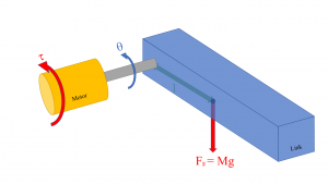
| [latex]\tau = I\ddot{\theta} + mgr\cos\theta + b\dot\theta[/latex] | (9.6) |
where [latex]I[/latex] is the scalar inertia of the link about the axis of rotation, [latex]m[/latex] is the mass of the link, [latex]r[/latex] is the distance from the axis of rotation to the center of gravity, [latex]g[/latex] is the gravitational acceleration, and [latex]b\dot{\theta}[/latex] is the viscous friction forces.
The equations of motion for a rigid body manipulator with multiple joints can be described by the Euler-Lagrange dynamics developed in chapter 5. Recall that the standard form of an n degree of freedom robot is
| [latex]M(q)\ddot{q} + C(q,\dot{q})\dot{q} + g(q) = \tau[/latex] | (9.7) |
Where [latex]q[/latex] is the joint variable vector, [latex]M(q)[/latex] is a nxn symmetric positive definite mass matrix, [latex]C(q,\dot{q})[/latex] is an nxn Coriolis/centrifugal matrix that is linear in [latex]q[/latex], [latex]g(q)[/latex] is an nx1 gravitational forces vector (that captures all the potential energy terms), [latex]\tau[/latex] is an nx1 generalized force vector made up of torques and forces. When the joint k is revolute, the kth component, [latex]\tau_k[/latex], is a torque acting around the joint axis [latex]z_{k-1}[/latex], while when the joint k is prismatic, the kth component is a force along the joint axis [latex]z_{k-1}[/latex].
9.3.2 Joint Space Motion Control
A common feedback controller for a singular actuator (single input) is a proportional-integral-derivative (PID) controller.
| [latex]\tau = K_p\theta_e(t) + K_i \int \theta_e(t)dt + K_D\dot{\theta}_e(t)[/latex] | (9.8) |
Where [latex]K_p[/latex], [latex]K_i[/latex], and [latex]K_D[/latex] are positive definite gain matrices, and is the error in the joint variable.
Rather than retroactively reacting to the robot’s movement through the errors, another strategy is to try and proactively generate the joint torques. This is done by utilizing a model of the robot dynamics and developing a feedforward torque by
| [latex]\tau = \tilde{I}\ddot{\theta}_e(t) + \tilde{h}\lgroup\theta_d(t),\dot{\theta}_d(t)\rgroup[/latex] | (9.9) |
Where [latex]\tilde{I}[/latex] and [latex]\tilde{h}[/latex] are based on the robot model. In an ideal scenario, the model would match the physical robot perfectly, i.e. [latex]\tilde{I} = I[/latex] and [latex]\tilde{h} = mgr \cos\theta + b\dot{\theta}[/latex].
There are two cases when it comes to considering multiple actuators (multi-input). Equation (9.6) generalizes the equations of motion for a robot with n joints. The first case is when the mass matrix, [latex]M(q)[/latex], is a diagonal matrix. This means that each join is independent of one another. Therefore, an independent controller can be applied to each joint as if they were singular actuators. This case is known as decentralized control. The second case is known as centralized control and is used when the joints are coupled (as in the mass matrix is not diagonal). The controller for this case is
| [latex]\tau = M(q)\lgroup\ddot{q}_d(t) + K_pq_e(t) + K_i\int q_e(t)dt + K_D\dot{q}_e(t)\rgroup + \tilde{h}\lgroup q_d(t), \dot{q}_d(t)\rgroup[/latex] | (9.10) |
9.3.3 Inverse Dynamics Control
Often these multivariable joint controls can be quite complex and nonlinear. The goal of using inverse dynamics is to find a nonlinear control law such that the feedback (when substituted into Equation (9.7) is a linear closed-loop system. In general, deriving a control like this might be difficult or near impossible. Fortunately, the problem is quite easy in the case of actuator dynamics since by inspection we can choose
| [latex]u = M(q)a_q + C(q,\dot{q})\dot{q} + g(q)[/latex] | (9.11) | |
| [latex]\tau = \tilde{I}\lgroup\ddot{\theta}_d(t) + K_p\theta_e(t) + K_i\int \theta_e(t)dt + K_D\dot{\theta}_e(t)\rgroup + \tilde{h}\lgroup\theta_d(t), \dot{\theta}_d(t)\rgroup[/latex] | (9.12) |
Equation (9.12) is a combination of the PID controller from Equation (9.7) with the model of the robot dynamics described by Equation (9.8). This controller consists of a feedforward from the robot dynamics plus a feedback linearization and is known as the inverse dynamics control. This results in the following double integrator system.
| [latex]\ddot{q} = a_q[/latex] | (9.13) |
Where [latex]a_q[/latex] is some control input yet to be chosen. This is very powerful since this means that each input can be designed to control a linear system. If we assume that [latex]a_{q,k}[/latex] is only a function of [latex]q_k[/latex] and its derivatives, then Equation (9.13) results in a set of n decoupled linear systems and the motions are independent of other links.
9.3.4 Task Space Motion Control
There are two options for a task space motion control with force/torque inputs: Convert to joint space trajectories and proceed with a joint space controller with force/torque inputs (covered in section 9.3.2). Or express the robot dynamics and control law in the task space. In this section, each method will be explored.
To convert to joint space, recall that the forward kinematics are given by [latex]X = f(q)[/latex] and [latex]\mho_b = J_b(q)\dot{q}[/latex]. To acquire the joint space trajectories, inverse kinematics is needed with the task space trajectories.
| [latex]q(t) = f^{-1}(X(t))[/latex] | ||
| [latex]\dot{q}(t) = J_b^\dagger(q(t))\mho_b(t)[/latex] | (9.14) | |
| [latex]\ddot{q}(t) = J_b^\dagger(q(t))(\dot{\mho}_b(t) - \dot{J}_b(q(t))\dot{q}_b(t))[/latex] |
The major drawback to this approach is that the inverse kinematics must be computed. Factors [latex]J_b^\dagger(q(t))[/latex] and [latex]\dot{J}_b(q(t))[/latex] can require significant amount of computer power – which may not be practical.
Recall Equation (9.7) which is the equations of motion for multiple actuators in joint space. By substituting [latex]\mho_b = J_b(q)\dot{q}[/latex] and [latex]\dot{\mho}_b = \dot{J}_b(q)\dot{q} J_b{q}\ddot{q}[/latex] into it, we can derive that the transpose inverse of [latex]J_b(q)[/latex] denoted as [latex](J_b^T)^{-1} = J_b^{-T}(q)[/latex]. Since [latex]F_b = J_b^{-T}\tau[/latex], it follows that
| [latex]F_b = \Lambda(q)\dot{\mho} + \dot{\eta}(q,\dot{q})[/latex] | (9.15) |
With [latex]\Lambda(q) = J_b^{-T}(q)M(q)J_b^\dagger(q)[/latex]. Equation (9.15) is the task space equations of motion and can be applied to the joint space controller derived in Equation (9.10)
| [latex]\tau = J_b^T(q)\lgroup\tilde{\Lambda}(q)\lgroup\dot{\mho}_d + K_pX_e + K_i \int X_e(t) dt + K_D\dot{X}_e\rgroup + \tilde{\eta}(q,\mho_b)\rgroup[/latex] | (9.16) |
Where [latex]\{\tilde{\Lambda},\tilde{\eta}\}[/latex] represents the controller's dynamics model.
9.4 Forced Control
9.4.1 Coordinate Frames and Constraints
Force control can be thought of as constraints imposed on the manipulator by the environment. For example, a manipulator moving through free space has no constraints and the force sensors would only detect the inertial forces. Now say the manipulator ran into a rigid object in the environment. While one or more degrees of freedom may be lost since the robot cannot move through the object, the robot will be able to exert a force onto the environment.
To describe the interaction between the robot and its environment, let the six-dimensional vector [latex]V[/latex] represent the instantaneous linear and angular velocity, i.e., [latex]V = (\nu,\omega)[/latex]. While the six-dimensional vector [latex]F[/latex] represents the instantaneous force and moment, i.e., [latex]F = (f,m)[/latex]. Let’s define the product of [latex]V \in SO(3)[/latex] and [latex]F \in SO^*(3)[/latex] by the usual way
| [latex]V \cdot F = V^TF = \nu^Tf + \omega^Tm[/latex] | (9.17) |
Say [latex]d_1, d_2, ..., d_n[/latex] are the basis vectors of [latex]SO(3)[/latex] vector space, and [latex]e_1, e_2, ..., e_n[/latex] are the basis vectors of [latex]SO^*(3)[/latex], then we say the basis vectors are reciprocal if
| [latex]d_ie_i = 0[/latex] if [latex]i \neq j[/latex] | ||
| [latex]d_ie_i = 1[/latex] if [latex]i = j[/latex] |
It is advantageous to write the product [latex]V^TF[/latex] in terms of the reciprocal basis vectors because it is invariant to a linear change of basis from one reciprocal coordinate system to another.
The compliance frame [latex]o_cx_cy_cz_c[/latex] is the frame in which the task can be easily described. This is to make the task specification simple. For example, a robot that is inserting a peg into a hole would have the compliance frame be where the peg was with the [latex]z_c[/latex]-axis along the cylinder axis. That way the task specification would be to insert the peg into the hole in the [latex]z_c[/latex] direction.
In the peg-and-hole robot example, Figure 9.2 represents the problem. The reciprocity condition is
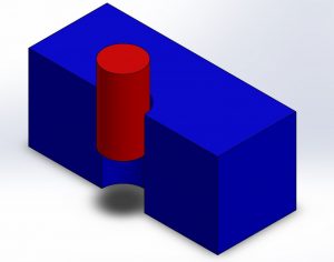
| [latex]V^TF = \nu_xf_x + \nu_yf_y + \nu_zf_z + \omega_xm_x + \omega_ym_y + \omega_zm_z[/latex] | (9.18) |
From Figure 9.2, it is clear that [latex]\nu_x = \nu_y = \omega_x = \omega_y = f_z = m_z = 0[/latex] and thus the reciprocity condition is satisfied. These relationships are known as the natural constraints since they arise from the environment.
The remaining variables [latex]f_x, f_y, \nu_z, m_x, m_y,[/latex] and [latex]\omega_z[/latex] are artificial constraints. They can be assigned reference values to be enforced by the control system. Say the speed of insertion of the peg in the z-direction is what is needed to be controlled, then an example of those artificial constraints would be [latex]f_x = 0, f_y = 0, \nu_z = \nu_d, m_x = 0, m_y = 0[/latex] and [latex]\omega_z = 0[/latex].
9.4.2 Task Space Control
It is natural to derive the control algorithm in the task space since typically the manipulator dynamics are given relative to the end-effector frame. Any interaction with the environment will cause forces and moments on the end-effector. Let [latex]F_{tip} = [f_x, f_y, f_z, m_x, m_y, m_z]^T[/latex] be a vector that represents the force and moment on the end-effector in that frame. When the end-effector is in contact with the environment, Equation (9.7) must be modified to include the reaction forces on the end-effector.
| [latex]M(q)\ddot{q} + C(q,\dot{q})\dot{q} + g(q) + J^T(q)F_{tip} = \tau[/latex] | (9.19) |
Typically, the robot moves very slowly. Thus, Equation (9.19) can be simplified to
| [latex]g(q) + J^T(q)F_{tip} = \tau[/latex] | (9.20) |
Consider the case where there are no sensors on the end-effector joint. In the absence of direct measurements, Equation (9.20) can be used to implement a force control law
| [latex]\tau = \tilde{g}(q) + J^T(q)F_d[/latex] | (9.21) |
Where [latex]\tilde{g}(q)[/latex] is the model of the gravitational torques and [latex]F_d[/latex] is the desired force/torques on the end effector. While this control law is quick and easy to implement, it relies heavily on a good model for the gravity compensation. Additionally, precise control over the torques produced in the robot joints is needed for this to work effectively.
An alternate strategy is to equip a six-axis force/torque sensor between the robot arm and the end-effector. This will allow for a direct measure of the end-effector wrench [latex]F_{tip}[/latex]. The best force control law for this scenario is a PI controller with a feedforward term and gravity compensation
| [latex]\tau = \tilde{g}(q) + J^T(q)\lgroup F_d + K_{fp}F_e + K_{fi}\int F_e(t) dt\rgroup[/latex] | (9.22) |
Where [latex]F_e = F_d - F_{tip}[/latex] represents the error between the desired end-effector force and the current end-effector force, [latex]K_{fp}[/latex] and [latex]K_{fi}[/latex] are positive definite proportional and integral gain matrices for the force control, respectively. This type of controller might be simple and appealing to use, however if applied incorrectly it can be potentially dangerous. If there is nothing for the end-effector to push against, it will accelerate in an attempt to create those forces to no avail.
Since most force control applications require little motion, we can limit the acceleration of the robot arm by adding a velocity damping term
| [latex]\tau = \tilde{g}(q) + J^T(q)\lgroup F_d + K_{fp}F_e + K_{fi}\int F_e(t) dt - K_{damp}\mho\rgroup[/latex] | (9.23) |
Where [latex]K_{damp}[/latex] is also a positive definite matrix.
9.5 Hybrid Motion/Force Control
As mentioned in the introduction, hybrid motion-force control is simply the sum of the two controllers expressed in task space. The task space motion controller (derived from the computed torque/force control law) and the task space force controller are each projected in their respective subspaces to generate the appropriate forces.
| [latex]\tau = J_b^T(q)\lgroup P(q) \lgroup \tilde{\Lambda}(q) \lgroup \dot{\mho} + K_pX_e + K_i \int X_e(t) dt + K_D\dot{X}_e \rgroup \rgroup + (I - P(q)) \lgroup F_d + K_{fd}F_e + K_{fi} \int F_e(t) dt + \tilde{\eta}(q,\mho_b) \rgroup \rgroup[/latex] | (9.24) |
Where [latex]P(q)[/latex] partitions the force space into the wrenches that address the motion control and those that address the force control. If the Jacobian is invertible, there will be no loss of generality. This will become clearer in the next chapter on Impedance control.
9.6 Conclusion
This chapter covers the concepts of motion control, force control, and hybrid motion-force control. As the names imply, motion control is concerned with building controllers so that the robot arm follows specified trajectories. Force control is concerned with building controllers so that the robot arm applies a desired force onto a surface. Lastly, hybrid motion-force control is concerned with combining the two types of control to produce both motion along a specified trajectory and a force on a surface.
Another important aspect of this chapter was the distinction between control using joint space and task space. Each has its advantages and disadvantages and it forces users to critically think about their robot application.
Practice Questions
9.1 Using the PID_Control_1joint.ttt file, design a PID controller in Python to move the link to the desired location. You're code should:
a. Prompt the user for the desired location (in degrees).
b. Prompt the user for the proportional, integral, and derivative gains.
c. The link should return to its original position when the script starts.
9.2 Using the inverseDynamics_Control.ttt file, design a PID controller plus inverse dynamics to move the link to the desired location. You're code should:
a. Prompt the user for the desired location (in degrees).
b. Prompt the user for the proportional, integral, and derivative gains.
d. Prompt the user for the target velocity.
c. The link should return to its original position when the script starts.
9.3 Repeat 9.1 and 9.3 in CoppeliaSim using sysCall_jointCallback(inData) in the Child Script. How does this compare to the solutions obtained in 9.1 and 9.3?
a. Add a graph so that the velocity of the joint variables is tracked.
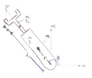
9.4 Given the RP manipulator below, what are the joint torques required to produce a force [latex]F = [3, 4]^T[/latex].
Solutions:
9.1 Can be found at the Github repository located here
9.2 Can be found at the Github repository located here
9.3 Can be found at the Github repository located here
9.4 The solution can be found here: 9.4 soln
References
Chung, W., Fu, L., & Hsu, S. (2008). Springer Handbook of Robotics - Ch. 6 Motion Control. Heidelberg, Berlin: Springer. https://users.dimi.uniud.it/~antonio.dangelo/Robotica/2012/helper/Handbook-mcontrol.pdf
De Schutter, J., Villani, L. (2008). Springer Handbook of Robotics - Ch. 9 Force Control. Heidelberg, Berlin: Springer. https://users.wpi.edu/~jfu2/rbe502/files/force_control.pdf
Hutchnson, S. Spong, M., & Vidyasagar, M. (2006). Robot Modeling and Control. PDF: John Wiley & Sons, Inc.
Kawasaki, H. (2009). Control, Systems, Robotics, and Automation vol. 22. Online: global Encyclopedia of Life Support Systems EOLSS. https://www.eolss.net/sample-chapters/C18/E6-43-38-03.pdf
