Navigation of Mobile Robots in Manufacturing Environments

Venkata Ravindhra Reddy Varikuti

5 Navigation of Mobile Robots in Manufacturing Environments

Venkata Ravindhra Reddy Varikuti

Chapter outline

5.1 Introduction

5.2 Model of Mobile Robots

5.2.1 Differential Drive Robots

5.2.2 Unicycle Model

5.3 Planning of Robotic Behaviors

5.3.1 Go to Goal

5.3.2 Obstacle Avoidance

5.3.3 Hybrid Automata

5.4 Navigation of Mobile Robots

5.4.1 Point and Circular Objects

5.4.2 Convex and Concave Objects

5.4.3 Boundary Following Method

5.4.4 Navigation of Differential Drive Robot

5.5 Summary

Practice Problems

Simulation

References

5.1 Introduction

Mobile robots have become increasingly popular in modern manufacturing environments due to their ability to automate repetitive and dangerous tasks, optimize production processes, and improve overall efficiency. However, effective control of mobile robots is critical to ensure their safe and efficient operation in these environments. Mobile robots can be used for material handling, inventory management, quality control etc. Control of mobile robots involves the development and implementation of algorithms that enable the robot to navigate, avoid obstacles, and perform tasks autonomously or under the supervision of an operator leveraging sensors and communication systems. The control system must also be able to adapt to changing environmental conditions and interact with other machines and systems in the manufacturing facility.

Mobile robots are typically categorized as either wheeled mobile robots (WMRs) or legged mobile robots (LMRs). In addition to these two types of ground robots, there are also autonomous underwater vehicles (AUVs) and unmanned aerial vehicles (UAVs) that fall under the umbrella of mobile robots. To ensure that these mobile robots can be controlled efficiently and effectively, it is necessary to have well-developed plans for both the motion of the robot itself and the environment in which it operates.

In general, there are three levels of robot planning, they are:

High level planning

High-level planning in robotics involves the generation of plans that specify the overall goals to be achieved by a robot. These plans typically involve a sequence of subgoals that need to be accomplished to achieve the overall objective. High-level planning is usually performed offline before the robot begins to execute its tasks. It can involve techniques such as task planning, task allocation, and mission planning.

Low-level planning

Low-level planning in robotics involves the generation of control signals to move a robot from its current state to a desired state. This can include tasks such as trajectory planning, motion planning, and path planning.

Execution level

The execution level in robotics refers to the lowest level of robot control, where the generated plans and commands are translated into actions by the robot’s actuators. This level involves the implementation of the low-level planning and control strategies that were developed in the earlier stages of robot planning. The execution level includes tasks such as motor control, sensor fusion, and feedback control.

In this chapter, we will provide a comprehensive overview of control planning in robotics (level 2) by developing robot navigation architectures for wheeled mobile robots (WMRs). We will also develop robotic behaviors that are more suitable for manufacturing logistics. First, we will develop the models of the most used WMR (differential drive and unicycle models) and then we will discuss the development of low-level planners (level 2), which are designed to guide control actions (level 3).

5.2 Model of Mobile Robots

Two of the most frequently used robotic models are the differential drive robots and the unicycle robots. In this chapter, we will delve into the kinematic models of these two robot types to gain a better understanding of their behaviors.

5.2.1 Differential-drive Robots

A differential drive robot is a type of mobile robot that has two wheels, with each wheel being independently driven by a motor. The motion of the robot is achieved by varying the speeds of the two wheels.

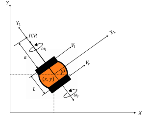
Figure 5.1. The geometry of differential drive WMR.

Created by Ravi Varikuti based on information from [2]

Assuming the robot is in a 2D plane with a wheel of radius $R$ , we can describe the robot’s motion using its position $\left( x,y \right)$ and orientation $\left( \theta \right)$ , and the velocities of its left and right wheels are $V_{l}$ and $V_{r}$ , respectively. The angular velocities of the right and left wheel being $\omega_{r}$ and $\omega_{l}$ , respectively. Using equations of motion for rotation, we can derive the following equations for the forward kinematics of a differential drive robot. All geometric parameters are illustrated in Figure 5.1.

We will find the velocity $\left(V\right)$ and angular velocity $\left( \omega \right)$ in the body frame of the mobile robot $\left( X_{1},Y_{1} \right)$ and use the forward kinematics to find velocities in the world frame $\left( X,Y \right)$ .

Let $a$ be the distance between the left wheel and the instantaneous center of rotation (ICR) and $L$ be the track width of WMR as shown in Figure 5.1. Let $\omega$ be the angular velocity of the mobile robot then,

Subtracting $V_{l}$ from $V_{r}$ and substituting $\omega$ in $V$ we get,

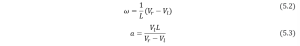
From (5.1) ,(5.2) and (5.3),

Assuming no slip between ground and wheels we can write,

From (5.4)and (5.5)

Let $\dot{x}$ and $\dot{y}$ are the velocities in $X$ and $Y$ directions respectively. $\dot{x}_{1}$ and $\dot{y}_{1}$ are velocities in $X_{1}$ and $Y_{1}$ directions respectively. By using coordinate transformation from frames {0} and {1} and substituting $\dot{y}_{1}=0$ , $\dot{x}_{1}=V$ we can write,

From (5.2), (5.6) and (5.7):

Although the differential drive model reveals the kinematics mechanism from wheel velocity control to the mobile robot position and orientation, it can be challenging for control design given the relatively complicated model and some robots may not have direct control over the wheels. As a simpler alternative, we will use the unicycle model, which describes the robot’s motion in terms of traditional velocity and angular velocity, rather than right and left wheel velocities. This simplified model will make it easier to analyze the robot’s kinematics and develop control strategies that enable the robot to perform its desired tasks.

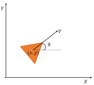
5.2.2 Unicycle Model

The motion of the robot is described by its position $\left( x,y \right)$ and orientation $\left( \theta \right)$ in a 2D plane. The unicycle model is illustrated in Figure 5.2.
The motion of the robot in the unicycle model is governed by two control inputs: linear velocity $\left( V \right)$ and angular velocity $\left( \omega \right)$ .

Created by Ravi Varikuti based on information from [1].

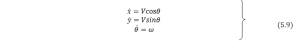
From Figure 5.2,

To connect the unicycle model with a differential drive robot, we can establish a mapping between the velocity and angular velocity of the unicycle and those of the differential drive robot. By doing so, we can effectively translate the motion of the unicycle into the motion of the differential drive robot and control it accordingly.

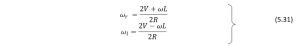
So, comparing (5.8) and (5.9), we get:

Solving for $V_{r}$ and $V_{l}$ in (5.10) and using (5.5):

Having developed a model of the robot, the next step is to incorporate behaviors into it that allow it to effectively navigate and interact with its environment. In the following section, we will focus on developing various behaviors for the robot, such as obstacle avoidance, goal-seeking, and path-following. These behaviors will be designed to work in tandem with the robot’s control algorithms, allowing it to adapt to different scenarios and achieve its goals. By combining these behaviors with the robot’s model and control algorithms, we can create a comprehensive navigation architecture that enables the robot to effectively operate in a real-world environment.

5.3 Planning of Robot Behaviors

Robot motions can be planned either offline (such as the A* and RRT* algorithms introduced in Chapter 4) or reactively online. For reactive robot behaviors, the robot needs to be equipped with onboard sensors to perceive the environment and react accordingly. To do so, we need to create a library of basic robot behaviors for the robot to select from based on the sensed environment. The two most basic behaviors of robots can be classified as follows.
1.Go-to-goal.
2.Obstacle Avoidance.

5.3.1 Go-to-goal

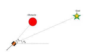
The main goal of mobile robot navigation in a manufacturing setting is to reach a specific objective, such as transporting goods or performing tasks like inventory monitoring and defect detection. The navigation process involves reaching a desired orientation and position. To achieve the desired orientation. To illustrate this concept, let us consider a simple scenario in which a mobile robot is moving at a constant velocity, denoted by $V_{o}$ as shown in Figure 5.3. The goal of the robot is to reach a specified location, and we will use the desired angle denoted by $\theta_{d}$ to achieve this objective.

By using the desired angle $\theta_{d}$ as a reference, we can develop control strategies that enable the robot to move towards the goal. The robot’s current orientation, represented by the angle $\theta$ , will be compared to the desired angle $\theta_{d}$ . Based on this comparison, the robot will adjust its angular velocity $\left( \omega \right)$ and head towards the goal.

Define the orientation error function as $e=\theta_{d}-\theta$ . To enable the robot to reach the goal, its direction should be aligned with the desired angle, ensuring that the error is zero. To achieve this, we need to design a controller that can guide the robot’s motion towards the goal. One simple controller can be used here is the PID (proportional-integral-derivative) controller. If 𝑢(𝑡) is control variable $K_{p}$ , $K_{i}$ , $K_{d}$ are proportional, integral and derivative gains respectively, then PID controller can be written as follows:

Figure 5.3 (a) Illustration for orientation control.

Figure 5.3 (b) Illustration for position control.

Created by Ravi Varikuti based on information from [1].

In this scenario control variable is $\omega$ ,

Note that when dealing with angular control, we need to pay special attention to the use of angles because they have a circular nature. For instance, angles of 0, 2π, 4π, etc. are equivalent in a circular sense. However, the PID controller will not be able to make the angular velocity zero for 2π or 4π.

To overcome this issue, we can use the atan2 function, which maps the robot’s position in Cartesian coordinates to an angle between π and -π.
Now we use atan2 function to define the new error $\left( p \right)$ as follows:

Using this $p$ as an error function in (5.13), we can ensure that the angular control signals generated by the PID controller are correct. By substitution of $p$ in (5.12), we get the angular velocity of the robot as,

To effectively operate mobile robots, it is essential to have control over both their orientation and position. While we have already developed a robot behavior for controlling orientation, we will now proceed to create a behavior that enables us to regulate the position of the robot.

consider the robot moving towards goal in direction towards the goal as shown in Figure (5.4). Assume the robot as point mass and system dynamics as

where $\boldsymbol{x}$ is the position and $\boldsymbol{u\left( t \right)}$ as control input.

Consider an example where the robot is moving in the direction towards the goal as shown in Figure 5.3 (b). $\boldsymbol{x_{g}}=\left( x_{g},y_{g} \right)^T$ are coordinates of goal and $\boldsymbol{x}=\left( x,y \right)^T$ are coordinates of robot as illustrated in Figure 5.3. Now we want to control the position of a robot, we will define distance between robot and goal as error function, therefore:

By taking control variable as velocity $V$ and substituting $e$ in PID controller Equation (5.12) we get:

From (5.16), (5.17) and (5.18) ( considering proportional controller for the sake of simplicity):

Now we have understood how to control both position and orientation of a point mass robot. We can use this position and orientation controllers to control the unicycle. By using the velocity in (5.18) and angular velocity in (5.15) and incorporating them in (5.9) we can control the robot.

In a factory environment, robots have to navigate through complex paths with obstacles present, which makes the navigation task much more challenging. Therefore, in addition to go-to-goal behavior, we need to develop more behaviors and planning algorithms that can help robots avoid obstacles and navigate to their destination safely and efficiently.

5.3.2 Obstacle Avoidance

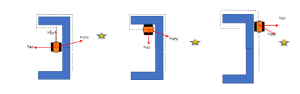
In the presence of obstacles, the task of reaching a goal becomes more challenging for a robot. To navigate through such environments, robots need to incorporate obstacle avoidance behaviors into their motion planning strategies. Let $\boldsymbol{X_{o}}$ , $\theta_{o}$ be position and direction of obstacle as illustrated in Figure 5.4.

Figure 5.4 Illustration of robot in the presence of obstacle.

Created by Ravi Varikuti based on information from [1].

To make robots reach the goal, let us think of some of the possible actions the robot can take and analyze the situation. Some of the possible actions that robot can take are shown in Fig 5.5.

Figure 5.5 (a) Robot moving away from obstacle

Figure 5.5 b) Robot is moving away from obstacle and towards goal.

Figure 5.5 (c) Robot moving towards goal.

Created by Ravi Varikuti based on information from [1].

In the case as depicted in Fig 5.5 (a) the robot is too cautious of the obstacle and moves away from the goal. In the second case (Fig 5.5 (b)), the robot was aware of the obstacle and directed towards the goal which can be a probable action. The third case (Fig 5.5(c)) was the direct go-to-goal action without sensing the obstacle. All kinds of actions are useful, depend upon specific situation. Let 𝑑𝑜 be the distance from the obstacle from where robot must be cautious and move away from it. We will define error function $\boldsymbol{e=X_{o}-X}$ . By taking the proportional part of controller we can write system dynamics as:

To navigate a robot, we must combine its go-to-goal behavior with its obstacle avoidance behavior. There are two main approaches for combining these behaviors: blended action and hard switching.
Blended action is achieved by assigning weightage to both behaviors. Figure 5.4(b) is an example of blended action. Let $\sigma_{1}$ and $\sigma_{2}$ be the weightage for go to goal and avoid obstacle behavior respectively. Then we can represent system dynamics as follows:

Blended behaviors are very helpful in achieving smooth behaviors but doesn’t guarantee in achieving desired motion.We can employ switching mechanisms for each behavior by specifying conditions of switching. For example, when robot is at distance less than 𝑑𝑜 use avoid obstacle behavior otherwise use go goal behavior. Hard Switching behaviors are good at achieving performance but also give bumpy ride due to abrupt switching.

Despite having pros and cons for each mechanism we can use both depending on the specific environment and objectives. In the next section, we develop generalized framework for this switching mechanism to order to model robotic behaviors.

5.3.3 Hybrid automata
We will now develop a general framework for switching mechanisms among different dynamic models of systems. Hybrid automata can be used to model systems that show both continuous and discrete behavior, such as robots that move and interact with their environment.

For example, a mobile robot that is programmed to navigate in factory environment may need to continuously monitor its sensors to avoid obstacles and make decisions based on the data it receives. The hybrid automata for this robot can have several modes or states, each representing a different behavior. For instance, the robot can have a “search” mode where it moves forward until it senses an obstacle, and then it can switch to a “turn” mode to navigate around the obstacle. In the “turn” mode, the robot can have two sub-modes, one for turning left and another for turning right. Each sub-mode can have a different set of continuous dynamics, such as different turning rates, to model the robot’s motion.

Let the continuous state of system be $\boldsymbol{x}$ and add a discrete state $\boldsymbol{q}$ because we’ll be transitioning between distinct modes of operation, then dynamics can be represented as follows:

To transition from one mode of operation to another in a hybrid system, certain conditions must be satisfied. These conditions are known as guard conditions. When a guard condition is satisfied, the system switches to a new mode of operation and a new set of dynamics and control laws become active. The transition occurs from $\boldsymbol{q}$ to $\boldsymbol{q'}$ if $\boldsymbol{x}$ $\in$ $\boldsymbol{G_{q,q'}}$ .

We would like to allow abrupt changes in the continuous state as the transitions occur which are called resets. Let the transition $\boldsymbol{x:=R_{q,q'}(x)}$ .

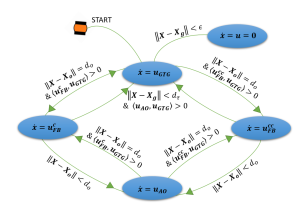
By combining all these together, we can get a model of Hybrid Automata (HA), which is illustrated in Figure 5.5.

Figure 5.6 The general structure of Hybrid automata.

Created by Ravi Varikuti based on information from [1].

To understand the HA model let’s consider the following example.

Consider a wheeled mobile robot moving on factory floor to deliver goods from one place to another with an obstacle present as shown in Figure 5.6. Now the robot must show two behaviors (go to goal and obstacle avoidance). To build Hybrid Automata, we need guard conditions. Let’s define guard condition in such a way that when the robot is away from the obstacle use go to goal behavior and when it is near to obstacle use avoid obstacle behavior. Let define 𝑑𝑑𝑜𝑜 be distance from the obstacle for switching behaviors. Let $X$ , $X_{g}$ , $X_{o}$ are the position of robot, goal and obstacle respectively.

From Section 5.3.1 and 5.3.2, we can write

For go to goal, $\boldsymbol{\dot{x}=u_{GTG}=}K_{GTG}\left\|\boldsymbol{X_{g}-X} \right\|$ ,
For obstacle avoidance, $\boldsymbol{\dot{x}=u_{AO}=}K_{AO}\left\|\boldsymbol{X_{o}-X} \right\|$ ,

Figure 5.7 Hybrid automata for go to goal and obstacle avoidance behavior.

Created by Ravi Varikuti based on information from [1].

Guard conditions: if $\left\| \boldsymbol{X_{o}-X}\right\|$ $\ge$ $d_{o}$ use go to goal behavior otherwise avoid obstacle behavior.
The hybrid automata model combining all dynamics and guard conditions are illustrated in Figure 5.6.

So far, we have seen only simple obstacles and tried to model the robot behaviors. Now we will try to include more complex obstacles and will develop a framework for the robot to navigate.

5.4 Navigation of mobile Robot

Up until now, we have only considered obstacles as point objects without considering their size or shape. However, the real world is filled with obstacles of various shapes and sizes. Therefore, it is necessary to incorporate obstacle avoidance behaviors for different shapes of obstacles to enhance the robustness of mobile robot navigation. The most commonly found obstacles can be modeled as a point, a circular object, a convex object, or a non-convex object.

5.4.1 Point and Circular Objects

We have already developed the model of a point object before in this chapter, the two behaviors: go-to-goal and obstacle-avoidance are sufficient to describe the motion of the robot. circular object can be described of point object at a center with sufficient safety radius. So, we can use go to goal and obstacle avoidance behavior we have developed for circular objects.

5.4.2 Convex and Non-convex Objects

A convex object is a shape that has no indentations or concavities. In other words, any two points on the surface of the object can be connected by a straight line that lies entirely within the object (see Figure 5.8(a)). Examples of convex objects include spheres, cubes, and cylinders.

In contrast, a concave object is a shape that has one or more indentations or concavities. This means that there are points on the surface of the object that cannot be connected by a straight line that lies entirely within the object (see Figure 5.8(b)). Examples of concave objects include bowls, cups, and vases.

(a) (b)

Concave object. Created by Ravi Varikuti based on information from [1].

Now let us try to navigate around a rectangle obstacle (convex obstacle) and try to model the robot behavior. We will use obstacle avoidance behavior ( $\boldsymbol{u_{AO}}$ ) as moving away from rectangle and go to goal behavior as moving towards goal. Figure 5.9 illustrates the motion of robot using the go-to-goal and obstacle avoidance controllers.

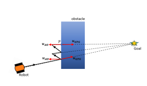
Figure 5.9 Illustration of robot trying to navigate around the rectangle.

Created by Ravi Varikuti based on information from [1].

From Figure 5.9 we can see that robot is moving towards the goal and avoiding obstacle until it reaches point 𝑝. At point 𝑝 we can see that that $\boldsymbol{u_{AO}}$ and $\boldsymbol{u_{GTG}}$ are in opposite directions and robot is oscillating to and forth at point $p$ , which is called Zeno phenomenon. This behavior is undesirable as it can cause the robot to become stuck in a loop or fail to reach its intended goal. It can also lead to instability in the robot’s control system and result in erratic behavior. So, we need to incorporate more behaviors into robot to address these problems. In the next section we will introduce boundary following behavior to address these problems.

5.4.3 Boundary Following Method.

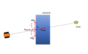
The objective of wall following behavior is to allow a mobile robot to track the shape of a wall or obstacle while moving towards a specific goal. To accomplish this, we can adjust the obstacle avoidance vector ( $\boldsymbol{u_{AO}}$ ) by rotating it either clockwise or counterclockwise by $\frac{\pi}{2}$ radians, resulting in a new vector $\boldsymbol{u_{FB}}$ that will align with the boundary. This provides the robot with two possible directions to follow the perimeter of the obstacle.

Let $\boldsymbol{u_{FB}^c}$ , $\boldsymbol{u_{FB}^cc}$ be the boundary following vectors when we rotate $u_{AO}$ in clockwise and counterclockwise direction respectively. This was illustrated in Figure 5.10.

Figure 5.10 Depiction of boundary following around rectangle.

Created by Ravi Varikuti based on information from [1].

Let $R$ be the rotation matrix and $\alpha$ be the scaling factor, then we can write:

Now we have two directions for robot navigate we need to specify conditions in such a way that is optimal for the robot to reach the goal. The decision regarding which direction the robot should move can be determined based on its tendency to reach the goal. This can be achieved by finding the angle between the vector $\boldsymbol{u_{FB}}$ and the vector $\boldsymbol{u_{GTG}}$ , which represents the direction towards the goal. The robot has tendency to move towards goal if angle between $\boldsymbol{u_{FB}}$ and $\boldsymbol{u_{GTG}}$ is less than $\frac{\pi}{2}$ (see Figure 5.9).

From linear algebra we know,

Therefore :

Although we have established a method for determining the robot’s direction of movement, we have not yet addressed the issue of when the robot should discontinue following the boundary and instead proceed directly towards the goal. While there is no definitive answer to this problem, we can attempt to model it by considering factors such as whether there is a clear path towards the goal and whether adequate progress has been made towards the target by following the boundary.

Consider the situations as illustrated in Figure 5.9.

Figure 5.10 (a)Robot at the time of switching to boundary follow behavior(b) robot following the boundary but moving away from goal(c)Robot having clear shot towards goal.

Created by Ravi Varikuti based on information from [1].

Let $\tau$ be time of last switching to boundary follow behavior, $\boldsymbol{ X}$ and $\boldsymbol{X_{g}}$ are position of robot and goal respectively. We can say progress towards goal have been made if,

In Figure 5.10(c), both the avoid obstacle behavior and go to goal behavior are driving robot towards goal. So, we can say we have clear shot towards goal when the angle between $\boldsymbol{u_{AO}}$ and $\boldsymbol{u_{GTG}}$ is less than $\frac{\pi}{2}$ .It can be represented mathematically as:

It is important to note that in Figure 5.10(b), although there is a clear shot towards the goal as per condition we stated in equation (5.27), the robot has not yet made sufficient progress towards reaching the target. So, to switch from boundary follow behavior we need to satisfy both Equations (5.25) and (5.27).

Now we have developed boundary following behavior to avoid obstacle. we will incorporate these behaviors into the hybrid automata model of mobile robot we have developed in section 5.3.3.

Let $d_{o}$ be the fixed distance from the obstacle for robot to exhibit boundary follow behavior. $d_{\tau}$ is the distance between robot and goal at the time of switching to boundary follow behavior. Let ϵ denote the minimum distance from the goal at which we consider the robot to have reached its destination.

Initially robot starts to move towards goal, the dynamics of the robot’s movement is governed by the “go to goal” behavior until it detects an obstacle at a distance $d_{o}$ , at which point it switches to “boundary following” behavior. The guard conditions for clockwise and counterclockwise navigation around the obstacle are determined by equation (5.25). When the robot switches to “boundary following” behavior, we will incorporate a reset to store the distance ( $d_{\tau}$ ) between the robot and the goal to calculate progress towards goal. As the robot follows the boundary and moves towards the goal, it will switch back to “go to goal” behavior once a clear shot to the goal has been identified and enough progress has been made. The guard conditions for this switching are governed by equation (5.26) and (5.27). If the robot moves beyond the distance $d_{o}$ from obstacle, then we will incorporate “obstacle avoidance” behavior to move towards the boundary. Once the robot reached goal we will stop. A complete hybrid automaton comprising all these behaviors have been illustrated in Figure 5.11.

Figure 5.11 Hybrid automata comprising go-to goal, obstacle avoidance and boundary following behavior.

Created by Ravi Varikuti based on information from [1].

The navigation architecture we have developed so far is based on the system model $\boldsymbol{\dot{x}=u}$ , where the control variable is the velocity. However, to apply this architecture to differential drive robots, we need to establish a way of connecting these modes.

5.4.3 Navigation of Differential Drive Robots

Figure 5.12 Navigation architecture for differential drive robot.

Created by Ravi Varikuti based on information from [1].

In Section 5.2, we developed kinematic models for differential drive robots and unicycle robots and subsequently integrated them. The control variables for differential drive robots are the velocities of the right and left wheels, denoted as $\omega_{r}$ and $\omega_{l}$ , respectively. In Section 5.3.2, we created a hybrid automaton that yields the velocity of the point mass robot. Now we will use This velocity as the reference velocity of the unicycle model, and we then use the methods outlined in Section 5.2.2 to compute the angular velocities of the differential drive wheels so that we can control the differential drive robot. This is represented in Figure 5.12.

Let the output from the Hybrid automation be $\boldsymbol{u=}$ $\left[ \begin{matrix} u_{1}\\u_{2} \end{matrix} \right]$ ,as we are taking $\boldsymbol{u}$ as a reference velocity the desired orientation will in point in the direction of $\boldsymbol{u}$ .

Therefore:

From Equations (5.9), (5.10) and (5.11) we can write:

By mapping two models by making a reference velocity as the unicycle velocity we get:

From Equation (5.9), we have:

Now we are equipped with the knowledge of input angular velocities, we can guide the robot toward its intended goal while ensuring that it avoids obstacles in its path. By applying these velocities, the robot can dynamically adjust its movements to safely navigate its environment and reach its destination.

5.5 Summary

Navigating an unstructured environment like manufacturing plant is a difficult task for robots and requires the implementation of advanced solutions developed over years of research. As robotics becomes increasingly utilized in such environments, it is important to continue building more behaviors to create more robust navigation systems. The chapter introduces basic behaviors for mobile robots, such as go-to-goal and obstacle avoidance behaviors and explains how these can be used to navigate the robot to a specific destination. The framework for switching between behaviors using hybrid automata is also introduced, providing a method for the robot to dynamically adjust its behavior based on changes in the environment. The chapter also addresses the challenge of navigating around convex obstacles, which are commonly present in manufacturing environments. Behaviors are developed for this task, which can be used in combination with other behaviors to create a complete navigation architecture for differential drive robots. The navigation architectures we have we have developed in this chapter can be used for many mobile robots such as drones, autonomous cars etc. by employing appropriate constraints.

Practice problems

1. Identify the convex and concave shapes from the shapes given below.

Created by Ravi Varikuti based on information from [1].

Solution: : Any two points on the surface of the object can be connected by a straight line that lies entirely within the object is convex object otherwise concave object. So, (a)and(b) are concave and (b) and (d) are convex. (See Figure 5.14 below).

Created by Ravi Varikuti based on information from [1].

2. What are the pros and cons of combining behaviors using hard switches and blending action?

Solution: The pros of hard switching are performance while that of blending action is smooth ride. The con of hard switches is bumpy rides and zero problems. The con of blended action is that there is no guarantee in achieving objective.

3. Consider a mobile robot navigating to warehouse to deliver goods at green check point from assembly line as shown in Figure 5.15. Using the navigation architecture, we had developed in this chapter and draw a trajectory of path followed by mobile robot.

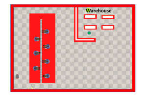
Figure 5.15 Mobile robot in factory space.

Created by Ravi Varikuti using Coppliasim.

Solution: The path of robot is shown in Figure 5.16 Robot will start moving towards goal and notices an assembly line and switches to boundary following behavior atby checking guard conditions for clockwise and counter clockwise boundary following and it moves along the wall until it has clear shot at then switches to go to goal behavior and moves towards goal and notices a wall and again switches to boundary following and follows the wall until it has a clear shot and reaches goal again by switching to go to goal behavior.

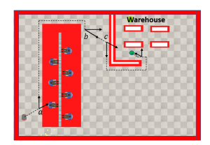
Figure 5.16 Path followed by mobile robot.

Created by Ravi Varikuti using Coppliasim.

Simulation

A simulation is done to showcase the go to goal, avoid obstacle and wall following behavior in coppliasim.

The coppliasim file and python script can be accessed through https://github.com/ClemsonSpring2023ME8930IntroRoboticsHRI/Ch5_Mobile_Robot_Control

References

[1] Magnus Egerstedt. ”Control of mobile Robots” course.

[2] Spyros G. Tzafestas.”Introduction to Mobile Robot Control”: Elsevier Inc,2014.

License

Icon for the Creative Commons Attribution-NonCommercial-NoDerivatives 4.0 International License

Advanced Robotics for Manufacturing Copyright © by Venkata Ravindhra Reddy Varikuti is licensed under a Creative Commons Attribution-NonCommercial-NoDerivatives 4.0 International License, except where otherwise noted.

Chapter outline

5.1 Introduction

5.2 Model of Mobile Robots

5.2.1 Differential-drive Robots

5.2.2 Unicycle Model

5.3 Planning of Robot Behaviors

5.3.1 Go-to-goal

5.4 Navigation of mobile Robot

5.4.1 Point and Circular Objects

5.4.2 Convex and Non-convex Objects

5.4.3 Boundary Following Method.

5.4.3 Navigation of Differential Drive Robots

5.5 Summary

Simulation

References

License

Share This Book