
8 Soft Robotics
Yalun Jiang
8.1 Introduction to Soft Robotics
8.2 Soft Robotic Modeling
8.2.1 Compliance of Soft Robots
8.2.2 Piecewise Constant Curvature Modelling (PCC)
8.2.3 Variable Curvature Modelling
8.2.4 Cosserat Rod and Euler Bernoulli Beam Theory Modeling
8.2.4.1 Cosserat Rod Theory Modeling
8.2.4.2 Euler Bernoulli Beam Theory Modeling with Relative States (EBR)
8.2.4.3 Euler Bernoulli Beam Theory Modeling with Absolute States (EBA)
8.2.5 Reduced-Order Modeling (ROM)
8.3 Impact and Contact Dynamics
8.4 Summary
-
- Practice Problems
- Simulation Code & Demo Animation Results
- References
8.1 Introduction to soft robotics
The birth of the modern computer science was in around 1950s, which boosted the development of robot industry. The first prototype of soft robots was proposed in 1960 to 1970s after the emergence of rigid robots and continuum robots. Largely restricted by the task space of the conventional purely rigid robots, engineers began to think about dividing a single segment of manipulator into several ones to increase its dexterity, which was called continuum robots, however not all the continuum robots are soft robots. Inspired by the creatures such as caterpillar, snake and the tail of sea horse, researchers have developed kinds of specific designs, such as cable driven, tendon driven, pneumatic actuated soft manipulators; the fundamental principles of the mechanism for cable and tendon driven soft manipulators are pretty similar, in most cases, we can see a combination of both. Cable driven ones usually will tie a very thin nylon, memory metal like Ti or some other high strength plastic material string to the end effector, and the rest part of the string will go along the backbone of the manipulator on its outer surface, to ensure that the manipulator will bend towards only one direction, several “tendons” will be mounted on the body of it. Usually to guarantee the manipulator can bend in the 3D space, at least 3 strings should be assembled onto it. When it is pulled on the base side, the extent (or angle) it bends depends how large the force we apply.

Created by Yalun Jiang based on the following images (a) “Swallowtail Caterpillar on Fennel Plant.jpg” by Watts, Flickr is licensed under CC BY 2.0 [1]. (b) “File:Big Sur Snake.JPG” by Jerry Marshall is licensed under CC BY-SA 3.0 [2]. (c) “File:Sea Horse.jpg” by CebuOceanParkCOP is licensed under CC BY-SA 4.0 [3].
However, it sounds like even for the cable driven robots, they still cannot get rid of “tendons”, so what is the unique part of tendon driven robots? The only difference between them is that for tendon driven ones, the number of strings is depending on how many tendons we use for each bending direction, each tendon is fixed with an individual string, and by pulling each string, only a certain portion of the manipulator will deform and this mode largely increase the flexibility and dexterity of its motion.
Pneumatic actuated manipulators are composed of hollow silicon rubber chambers, when being pressurized with pressure supplies, due to the elastic property of the rubber, each chamber will bend and be stretched at the same time (usually the bending rate will be much larger); and similar to the two modes mentioned above, at least three chambers can guarantee an overall range motion. To achieve the similar effect of tendon driven robots, one direction bending is determined by two parallel smaller chambers in pairs with sleeve surrounding its outside, the classic example is McKibben muscle. Or the dimension is identical for all the segments, inside the chambers there are thinner tubes with different length starting from the base. For instance, if we have two segments for a single soft robot arm, we assume and label each segment as 1 and 2 from the base to the end effector, to control the distal arm (No. 2), there must be a power source tube go through segment 1 and 2, and to pressurize segment 1, a shorter tube will be assembled in it as well; the portion reaching the joint of both segment is well sealed so that each tube will be responsible for controlling one single segment, the mechanism can be seen in the figure below.
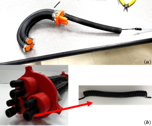
Created by Yalun Jiang based an adaption of information and images from [4]
Since soft robots have much more advantages over traditional rigid ones, such that for some compact working areas or the environment is fragile like minimally invasive surgery, it will be hard for the rigid ones to reach or can easily destroy the tissue like cytomembrane of blood vessels, it’s necessary for us to do more study and research in this field. The following sections of this chapter will focus on the main stream modeling methods, the popular contact and impact problem between soft and rigid objects and some related simulations.
8.2 Soft Robot Modeling
8.2.1 Compliance of Soft Robots
When talking about soft robots, we must talk about their compliance. Lots of books forgot to propose such concept at the very beginning, or put it to the very behind of the book after introducing the dynamics. You may ask what is compliance? Why must we mention the concept of compliance along with soft robotics? Actually compliance denotes the executive capability of the manipulator under certain external forces or any other types of input sources, let us consider two identical soft manipulators exerted with the same amount of input at the same position, i.e., 5 N towards the positive x axis on the end effector. We assume the anticipated displacement of the end effector is 2 m. However, in reality, the end effector of manipulator 1 can reach 1.8 m, and that of manipulator 2 can reach 1.5 m. We can say that the compliance performance of manipulator 1 is better than that of 2.
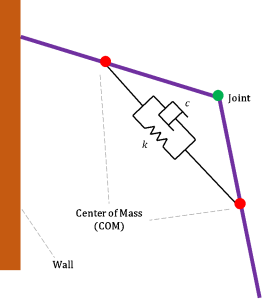
In recent years, the compliance of robots is much more relevant to their ability in human-robot collaboration and robot-environment interaction. Even the conventional rigid robots can still handle jobs like grasping eggs. However, too large or too small force applied will either cause the egg being cracked or falling down onto the ground. Thus compliance is not a feature just belongs to soft robots. When equipped with force sensors, even the rigid robots can do some assembly tasks precisely. When speaking of soft robots, their material properties contribute a lot to the advantages over rigid ones in terms of compliance, and meanwhile if extreme conditions really happened, the material itself will act like a buffer (we can simply assume it as a mass-spring-damper system as shown in the figure below) to protect the humans from being directly injured, which makes them more suitable for work that collaborating with humans.
Created by Yalun Jiang
However, the non-uniformity of the material when manufacturing makes the motion of soft manipulator hard to predict, so the main stream control strategies are impedance control (to treat the contact and impact problem as mass-spring-damper system), force control, position control and hybrid control. The contents for this chapter are scheduled as follows: firstly we shall introduce some fundamental principles of general modeling theories and methods, constant curvature, Cosserat Rod and Euler Bernoulli Beam Theory; after that, we are going to briefly discuss the general thoughts of up-to-date modeling methods based on the primary theories, such as Euler Bernoulli Beam Theory with relative and absolute states (EBR and EBA) and Reduced-Order Modeling.
8.2.2 Piecewise Constant Curvature
(1). Fundamental Principles
The Piecewise Constant Curvature Theory (PCC) is the most commonly used modeling method for both continuum and soft robots , just as its name implies, no matter to what extent we bend or twist the arm, we ignore its uneven extension along the axial direction (or backbone) which means that the length change per unit length due to deformation is deemed to be a constant in a certain portion or range of the arm. The novelty of this modeling method is that we do not have to spend so much time on struggling with the property of material itself and complex mechanical property due to its natural heterogeneity, instead its geometry factors will be our main focus. Since lots of more advanced deuterogenic modeling methods (e.g. Piecewise Variable Curvature) were modified and refined based on this assumption, understanding the basic principles of this method is vital.
Before we formally introduce the details about modeling process, let us have an overall knowledge about its limitations and specific application scenarios, and also clarify the definitions of all the variables involved.
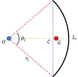
As shown in the figure below, we use an example of soft robot arm (SRA) to illustrate it. The rule for setting up the coordinate frame is similar to the Denavit-Hartenberg (D-H) convention. The SRA is a closed tube surrounded by the green boundaries in a cylinder shape, whose length is l. The bending angle θ is computed based on the plane (in blue) the SRA forged after deformation. And then the twist angle ϕ will be established based on the angle between the bending existing plane (the blue plane we have just mentioned) and the plane xoz, using the right-hand rule. The anti-clockwise direction will lead to a positive angle change.
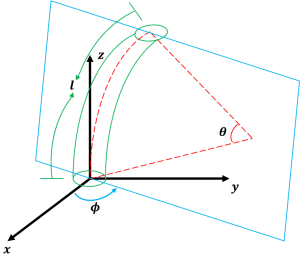
Created by Yalun Jiang
In terms of the material property itself, compared with solid metals we would commonly see, such as steel, the slope of the stress-strain curve of SRA before the elastic and yield limit points is not a constant. Furthermore, its yield limit point usually comes earlier than metals’, which makes the extension rate so unpredictable with the increasing external load exerted on the soft materials. More specifically, in practical applications, the curvature will not be a constant for larger bending angles, and the error will become even more significant when the external load has exceeded the yield strength. Therefore, the constant curvature theory only applies when the bending angle change is small (within 10°) with respect to the stationary state. That is the reason why the PCC method is introduced. Just like Newton Leibniz’s integration method, we can cut an SRA into multiple equal-length portion and treat each of them as a unit element, and apply CC (constant curvature) for each one so that we will obtain a more accurate simulation results compared to that with the CC assumption on the full range of SRA. When the unit element is small enough, here brings another research field, finite element analysis (FEA), which is not our focus on this section, we will cover it in Section 8.2.4.
(2). Mathematical Modelling
To start with, and make the readers have a better understanding about the modelling quickly, we are going to work on a 2D example first. Similar to the Fig. 8.5, we consider a scenario that there is an SRA attached onto a wall. Now we are facing the front view of the system as shown in Fig. 8.5 below. We assume there is no movement along the positive or negative z_0 axial direction so that it will completely become a 2D problem. To make the model more general, we apply a subscript for all the variables to denote the ith arm, to finally derive the dynamics of the system. We firstly have to start from the kinematics of the end effector using forward kinematics, then we can estimate the kinematics of the centre of mass (COM) of the arm.
Created by Yalun Jiang
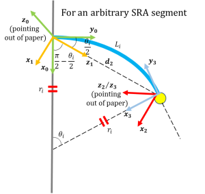
To ensure that the frame of the next arm’s joint corresponds to the former one (in our case, it’s frame 0,  ), though there seems to be only one link (the chord), we have to make it into 3. Here we would not spend too much space to discuss about the frame set up in D-H convention (for more details, please check [5]), since it has been covered in the very front chapters, we assume you already get familiar with this. After setting the frames, the D-H parameter table is given as follows.
Table 8.1 D-H parameter table for example shown in Fig. 8.6

where  is the chord length that can be computed using Pythagorean theorem.
According to the homegeneous transformation matrix rule, we have a general formula that
where  and
and  represent for revolution and translation respectively,
  is the angle rotated around
  axis,
axis,  and
and  can be seen as the translation distance along and
  axis,
axis,  is the angle rotated around axis, so we can derive the matrix for each link as follows,
![\therefore\ H_1^0=\left[\begin{matrix}\cos{\left(-\frac{\theta_i}{2}\right)}&-\sin{\left(-\frac{\theta_i}{2}\right)}&0&0\\\sin{\left(-\frac{\theta_i}{2}\right)}&\cos{\left(-\frac{\theta_i}{2}\right)}&0&0\\0&0&1&0\\0&0&0&1\\\end{matrix}\right]\left[\begin{matrix}1&0&0&0\\0&\cos{\left(-\frac{\pi}{2}\right)}&-\sin{\left(-\frac{\pi}{2}\right)}&0\\0&\sin{\left(-\frac{\pi}{2}\right)}&\cos{\left(-\frac{\pi}{2}\right)}&0\\0&0&0&1\\\end{matrix}\right]=\left[\begin{matrix}\cos{\frac{\theta_i}{2}}&\sin{\frac{\theta_i}{2}}&0&0\\-\sin{\frac{\theta_i}{2}}&\cos{\frac{\theta_i}{2}}&0&0\\0&0&1&0\\0&0&0&1\\\end{matrix}\right]\left[\begin{matrix}1&0&0&0\\0&0&1&0\\0&-1&0&0\\0&0&0&1\\\end{matrix}\right]=\left[\begin{matrix}\cos{\frac{\theta_i}{2}}&0&\sin{\frac{\theta_i}{2}}&0\\-\sin{\frac{\theta_i}{2}}&0&\cos{\frac{\theta_i}{2}}&0\\0&-1&0&0\\0&0&0&1\\\end{matrix}\right]](https://opentextbooks.clemson.edu/app/uploads/quicklatex/quicklatex.com-c8dacf6b87d40c1c36d5ccdf7490d89b_l3.png "Rendered by QuickLaTeX.com")
![H_2^1=\left[\begin{matrix}1&0&0&0\\0&1&0&0\\0&0&1&d_2\\0&0&0&1\\\end{matrix}\right]\left[\begin{matrix}1&0&0&0\\0&\cos{\frac{\pi}{2}}&-\sin{\frac{\pi}{2}}&0\\0&\sin{\frac{\pi}{2}}&\cos{\frac{\pi}{2}}&0\\0&0&0&1\\\end{matrix}\right]=\left[\begin{matrix}1&0&0&0\\0&1&0&0\\0&0&1&d_2\\0&0&0&1\\\end{matrix}\right]\left[\begin{matrix}1&0&0&0\\0&0&-1&0\\0&1&0&0\\0&0&0&1\\\end{matrix}\right]=\left[\begin{matrix}1&0&0&0\\0&0&-1&0\\0&1&0&d_2\\0&0&0&1\\\end{matrix}\right]](https://opentextbooks.clemson.edu/app/uploads/quicklatex/quicklatex.com-283460d8f60c2e4b568a87bf843346aa_l3.png "Rendered by QuickLaTeX.com")
![H_3^2=\left[\begin{matrix}\cos{\left(-\frac{\theta_i}{2}\right)}&-\sin{\left(-\frac{\theta_i}{2}\right)}&0&0\\\sin{\left(-\frac{\theta_i}{2}\right)}&\cos{\left(-\frac{\theta_i}{2}\right)}&0&0\\0&0&1&0\\0&0&0&1\\\end{matrix}\right]=\left[\begin{matrix}\cos{\frac{\theta_i}{2}}&\sin{\frac{\theta_i}{2}}&0&0\\-\sin{\frac{\theta_i}{2}}&\cos{\frac{\theta_i}{2}}&0&0\\0&0&1&0\\0&0&0&1\\\end{matrix}\right]](https://opentextbooks.clemson.edu/app/uploads/quicklatex/quicklatex.com-15b6ed006ed84b6d08abb702f0976239_l3.png "Rendered by QuickLaTeX.com")
![\therefore H\left(\theta_i\right)=H_1^0H_2^1H_3^2=\left[\begin{matrix}\cos{\frac{\theta_i}{2}}&0&\sin{\frac{\theta_i}{2}}&0\\-\sin{\frac{\theta_i}{2}}&0&\cos{\frac{\theta_i}{2}}&0\\0&-1&0&0\\0&0&0&1\\\end{matrix}\right]\left[\begin{matrix}1&0&0&0\\0&0&-1&0\\0&1&0&d_2\\0&0&0&1\\\end{matrix}\right]\left[\begin{matrix}\cos{\frac{\theta_i}{2}}&\sin{\frac{\theta_i}{2}}&0&0\\-\sin{\frac{\theta_i}{2}}&\cos{\frac{\theta_i}{2}}&0&0\\0&0&1&0\\0&0&0&1\\\end{matrix}\right]=\left[\begin{matrix}\cos{\frac{\theta_i}{2}}&\sin{\frac{\theta_i}{2}}&0&d_2\sin{\frac{\theta_i}{2}}\\-\sin{\frac{\theta_i}{2}}&\cos{\frac{\theta_i}{2}}&0&d_2\cos{\frac{\theta_i}{2}}\\0&0&1&0\\0&0&0&1\\\end{matrix}\right]\left[\begin{matrix}\cos{\frac{\theta_i}{2}}&\sin{\frac{\theta_i}{2}}&0&0\\-\sin{\frac{\theta_i}{2}}&\cos{\frac{\theta_i}{2}}&0&0\\0&0&1&0\\0&0&0&1\\\end{matrix}\right]=\left[\begin{matrix}\cos^2\frac{\theta_i}{2}-\sin^2\frac{\theta_i}{2}&\cos{\frac{\theta_i}{2}}\sin{\frac{\theta_i}{2}}+\sin{\frac{\theta_i}{2}}\cos{\frac{\theta_i}{2}}&0&d_2\sin{\frac{\theta_i}{2}}\\-\sin{\frac{\theta_i}{2}}\cos{\frac{\theta_i}{2}}+\cos{\frac{\theta_i}{2}}\left(-\sin{\frac{\theta_i}{2}}\right)&-\sin^2\frac{\theta_i}{2}+\cos^2\frac{\theta_i}{2}&0&d_2\cos{\frac{\theta_i}{2}}\\0&0&1&0\\0&0&0&1\\\end{matrix}\right]](https://opentextbooks.clemson.edu/app/uploads/quicklatex/quicklatex.com-abad3940803763446764c6df78ca873e_l3.png "Rendered by QuickLaTeX.com")

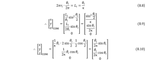
And we all know that the first three elements in the last column of the homogeneous transformation derived above, the coordinate the end effector will be

Then the COM of the arm can be deemed to coincide with the geometry center of the chord, so we have

Some related proof can be seen as follows,
According to the definition of COM of an arc shape, we have the distance between its COM and the center of complete circle below,

Created by Yalun Jiang
where point  is the COM of the arc and point
  is the geometry center of the generalized chord,
  is the curvature radius. The length of OC should be
  ,
,  .
.
Thus the gap between point and will be

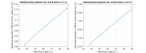
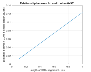
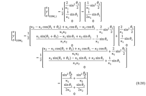
We performed two groups of control simulations based on the variation of bending angle ( ) and length (
 ) of SRA segment. The results showed that the length of SRA domains the distance between COM of SRA and center of SRA chord when suffering from a bending torque/force, further influences the accuracy of the model.
 &
&  when
when  and
and  respectively.
 & when
  .
.Created by Yalun Jiang
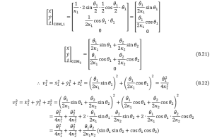
To evaluate this approach of simplified modeling, the length of each segment of SRA has been measured, approximately as shown in the figure below, and the simulation results aforementioned showcased that even for large bending angle ( ), the magnitude of is very small. The authentic inertia tensor (adding this part by using inertial parallel theory) would not differ such a lot from that of the simulation model, which indicates that the current model is reliable depending on the length of SRA. In the future, if we plan to study the dynamics of longer SRA, we can divide each segment by multiple equal length cylinder bars (RPR manipulator, R: revolute, P: prismatic ) to improve its accuracy.
Back to our kinematics, the linear velocities of the COM in the three axial directions will be the derivative of the coordinate,

Since the arc length or the arm length  changes with the bending angle , to ensure there is only one variable in the expression, we shall express with the constant curvature
  and which is showcased as follows,
If we only consider about the linear velocities of the system, and take the zero potential plane as plane , the kinetic and potential energy of the system can be summarized as follows,
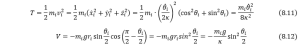
Using the Euler-Lagrangian Equation, we can forge the Lagrange’s function as

Thus the governing equation of the system will be

where  is the torque supplies exerted on the COM of the arm
  . In the following sections, we would not spend time on derivation of the dynamics individually, as the procedures are basically the same, instead we will focus more on the theorems themselves.
And for 3D case, we just need to add another rotation matrix  , which is forged by the manipulator twisting about axis, by pre-multiplying Eqn. (8.2), the homogeneous transformation matrix for 3D problem of the joint will be
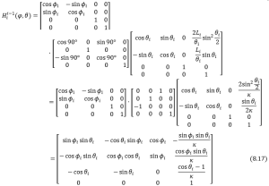
Then we just need to plug it in using the same procedure from Eqn. (8.3) to obtain the motion equations for 3D problems.
8.2.3 Variable Curvature Modelling
As stated previously, to deal with the limitation of the PCC method that the simulation accuracy will largely be affected by the length and bending angle of the SRA, the Variable Curvature (VC) modelling was designed to elminate such influence as much as possible. The core principle of VC is to separate the whole arm into different segments (the length, diameter and material properties for them might be different), for each one we can assign a unique curvature . Still we can use exactly the same example as we used in the last section. The only difference is that this time, we are going to add a secondary arm onto the joint (or end effector) of the first arm. To distinguish their paramters, we set the bending angles as  and
and  , the curvatures are
  and
and  , the arc lengths are
  and
and  .
.
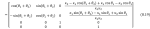
The homogeneous transformation matrices for the first joint and the new end effector (of arm 2) can be derived from experienced formulas that
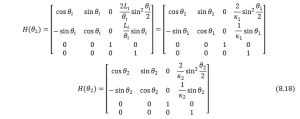
Thus the homogeneous transformation matrix for the end effector will be expressed as

Then the coordinates for COM of each arm will be
Again using direct derivative method, the linear velocities of each COM can be computed as follows,

For simple 2D problems, we can use propagation method [6] to compute the angular vecloties of the COMs; for linear velocities, we can also use the Jacobian matrix which is shown by the example in Eqn. (8.24) below

Using all the equations and expressions derived so far, we can assembly them all into the Lagrange’s Equation and finally obtain the motion equations of the whole system, then with proper initial conditions and settings for the ODE solvers, we can do simulations according to our requirements.
8.2.4 Cosserat Rod and Euler Bernoulli Beam Theory Modeling
To guarantee a more accurate simulation result, we could separate a complete SRA into more and more segments with different curvatures assigned as we discussed in Section 8.2.2 and 8.2.3. When the quantity of the segments is large enough or the size of each segment is small enough, the problem will become FEA. However, FEA is more adaptable for statics. The computation cost and efficiency for a dynamic process make it not applicable for real time simulation and control [6]. So for continuum robots or SRAs, here we would like to introduce another classification of modeling method which is based on Cosserat Rod and Euler Bernoulli Beam Theory and can depict the mapping between force/torque input and manipulator’s configuration directly.
To begin with, let us first take a quick review about the fundamental principles. For a beam or rod with an even shape (which means that no matter what the shape or the dimension of the cross section area, they are identical along its length when stationary), we can always make the following assumptions [7] to simplify our problem:
- The shape and dimension of the cross section area will not be changed no matter for what magnitude the external load exerts;
- The cross section plane at any portion of the beam will always be perpendicular to the neutral axis (it is exactly the same concept as backbone in the soft manipulator area);
- The elasticity for the beam or rod is identical at any point, or it can be seen as an ideally linear spring.
For Cosserat Rod Theory, the assumptions can be slightly different, which can be seen as follows:
- The first application scenario of this theory is the length of the rod () is much larger than its diameter (
 ), or the dimension of the cross section area can be ignored, i.e.,
  , and sometimes we can directly treat the rod as a line in the 3D space for simplification;
 - It has two coordinate frames for this system, one of them is the global coordinate frame, which is composed of three pairs of mutually orthogonal unit vectors
 . Another is a local one
  which is directly related to the length of the arc
  . The biggest difference from Euler-Bernoulli Theory is that the plane forged by the two local unit vectors
  and
and  doesn’t have to be perpendicular to the tangential line of the curve (because we can see the rod as a line as stated in the previous assumption) all the time because sometimes there will be some shear force at length ;
 - The continous differentiability of the curve is not necessary.
The common thing of both modeling methods is that the orientation and the position of the end effector plane in the 3D space can be expressed by similar three mutually orthogonal unit vectors so that the relationship between the moment and the shape of the rod can be mapped.
8.2.4.1 Cosserat Rod Theory Modeling
Using Fig. 8.10, we can continue to define the following concepts and variables:
- : Tangent, stands for the tangential unit vector of the curve
 : Normal, stands for the normal unit vector of the curve
 : Binormal, stands for the binormal unit vecotr of the curve
We assume that the shape function of the rod curve is  , where is the lengh of the arc (
![s\in\left[0,L\right]](https://opentextbooks.clemson.edu/app/uploads/quicklatex/quicklatex.com-1dafb1da5efd3ab692f4ab2ee1c52e34_l3.png "Rendered by QuickLaTeX.com") ), then the three unit vectors can be expressed as
), then the three unit vectors can be expressed as

Nevertheless, it’s still hard and not sufficient to explain the interconnections between the external force/torque and deformation. So next we will divide the problem into three steps: figure out how internal strain affects the shape of the rod, compute the resultant internal strain caused by external load and finally clarify the relationship between the internal strain between tensile & shear stress [8].
As aforementioned, the configuration of the rod  is determined by the orientation of a certain point and its position in the 3D space , but none of those can be associated with strains. The motion of the rod can be classified as rotation and translation, the rotation about the local three unit vectors will cause bendings in two directions , and one torsion along the curve axis direction . The nature of all the three variables is the angle change (or angular velocity) that vary about arc length . Among them, the first two depict the bending strain rate (the curvature) and the last one illustrates the torsional strain rate; for the translation, correspondingly it will cause shear stress in two local unit vector directions and , and one tensile stress (extension) . For simple kinematics problem, we have such relationship between linear and angular velocity , where is the path vector pointing from the rotational axis to the position the object locates at the current time instant. Similarly, we establish the differtiation equations as follows,

where  .
.
Then we need to map how the external force would affect the magnitude of the internal strain of the rod. From the figure below, we can determine the strain for the whole rod by integration about the length, from the zoom-in diagram, we have the following equations,

where  is the arc length measured from the origin to an arbitrary position,
 and
and  are internal and external forces exerted on the rod respectively, and
  and
and  are the moments acting on the rod internally and externally. The external force and moment and are evenly distributed along the length of arc. If we compute the total force or moment from the origin (or the position where the rod is attached or fixed), we just need to replace in the bracket with 0, and by differentiating both equations above, we can obtain

Next we shall derive the interconnection between the strain and stress according to the property of the material used for the rod, which can be seen as follows,
where  and are constant, and represent Young’s modulus and shear modulus respectively..
 ,
,  and
and  are the cross section area, moment of inertia and polar moment of inertia at an arbitrary arc length .
  and
and  are the internal strains calculated related to the reference frame.
Then we can bound all the three parts together to obtain 4 differential equations, from Eqn. (8.27) to (8.30) about the orientation, position, force and moment respectively, thus the problem will be solved as below,
![]()

8.2.4.2 Euler Bernoulli Beam Theory with Relative States (EBR)
The following three parts will not involve so many equations or formulas derivation, since they are more like new generation algorithms which are far away from the most fundamental principles of modelling methods stated above. So here we just would like the readers to know a rough knowledge and concept of modern methods through literature review.
Through the study about PCC and Cosserat Rod Theory, we can establish our model either continuously (differentially) or discretely depending on specific application scenarios, and they will become the two main branches for development of soft manipulator modelling in the future. Considering the computation cost and real time simulation efficiency, sometimes we have to make secondary assumptions on basis of the modelling theory we use to simplify our model. The subsequent three methods will be good examples of simplification. Among them, the methods that Euler Bernoulli Beam Theory with relative states (EBR) and absolute states (EBA) are the versions aiming to solve discrete models. For the Reduced-Order Method, it was designed to model continuum robots.
The common point of all the three methods is to use quarternions to express the orientation  and position
  of an arbitrary arc length in the 3D space. As shown in the Fig. 8.9, the blue dots could be deemed to be the joints of soft manipulator. The angle change
  and the extension
  (not shown in the diagram) are measured under the local frame (the green segment). For example, is the angle between the tangential line of the previous segment curve (the red section) and the straight line connecting the current and the next joint. The extension is compared to the unstretched state of the green section. All the quarternions can be expressed using and , based on the mapping between force or torque supplies and the space configuration of manipulator, so that we can compute the bending moment and shear force and vice versa.
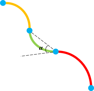
(Created by Yalun Jiang based on information from [10])
8.2.4.3 Euler Bernoulli Beam Theory with Absolute States (EBA)
Similar to EBR, the manipulator states are measured based on a global coordinate frame, which could be located at the position the base is fixed, or somewhere else in the 3D space. In terms of the simulation results, EBA performs better than EBR in dealing with nonlinearities. However, the stability and reliability for larger shear force and longer manipulators were not so good.
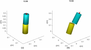
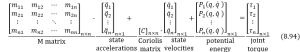
To test the performance of EBA modelling method, can use the TMTDyn [9] simulation package (source code can be found on GitHub: https://github.com/smhadisadati/TMTDyn). In the Simulation section of this chapter, we will talk more details about it. For a manipulator with multiple segments, when suffering from a larger external load, the adjacent segments which are supposed to be connected tightly with each other will be separated apart. To verify this, firstly we can apply 0.5 N force along x direction on the SRA tip without any other pressure input, the package could successfully run without error and the separating problems did not occur for this situation as shown in Fig. 8.10(a). However, when the force input was increased to 5N as shown in Fig. 8.10(b), the deformation is about the maximum at about simulation time 13.5 s. We found that the separating situation still exists for large shear force, but not that obvious since we have set the Young’s Modulus four times as the original value, which also indicated that Young’s Modulus dominates the performance of animation except for geometry factors of the SRA.
Created by Yalun Jiang
So we can make a rough conclusion based on the results so far. The discrete modeling method (taking a whole SRA as several rigid links) like EBR and EBA might not be a proper way to show the properties of SRA deformation for large shear force. In the next section we will try other modeling method in the package to see if there would be any improvement.
8.2.5 Reduced-Order Modeling Method (ROM)
The Reduced-Order Modeling Method is firstly derived to solve the dynamic problem of pneumatic chamber actuated manipulator, since it is hard to use a specific formula to map the relationship between pressure supplies and the generalized force/torque produced by the manipulator (because most of the research achievements just focused on the experimental data merely) [12, 13, 14]. To make it more meaningful for practical use, the orientation  and position
  can be expressed by a Lagrange polynomial series in the format as shown below,

where  is the number of the system’s order. It is worth-noting that is not identical to the number of segments used in other modelling methods like EBA and EBR, though they can achieve basically the same effect, i.e., the larger the number, the more accurate results we will obtain.
 is a coefficient matrix for the polynomial whose size is determined by the number of . In the simulation package, it will act as the state variable.
 is the shape function of the manipulator. To understand what is the meaning by “reduced-order” , we choose two “measurement” planes, one is rightly in the geometry middle of the manipulator and another is located at the end effector. If we are using Cosserat Rod Theory, to map the configuration of the manipulator, we need the position and orientation both the middle and end effector plane (the order is deemed to be 2), however, for ROM, we only need the information about the middle plane and an orientation vector pointing from the middle one to the end effector. Thus the order of the system can drop from 2 to 1, we can say that the order is reduced.
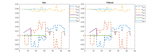
To compare the performance of different methods , we should apply exactly the same conditions, 5N force exerted on the SRA tip with 4 times of original Young’s Modulus value (480 GPa). The results can be seen in the Fig. 8.11. We can find that with the same input, the maximum displacement in x direction for EBR and ROM methods are about 0.25 m and 0.13 m respectively, which is a huge difference. There is some relative explanation in the research paper of the TMTDyn simulation package. It says for static motion (no external force on the tip) when the number of segments was set to be very small, like 1 or 2, the absolute and normalized error for ROM is smaller than EBR and EBA; however, with the increasing of numbers of segments, the accuracy of EBA and EBR will rapidly improve. But for the cases with external loads, the ROM modeling method remains the best accuracy among all the methods.
Created by Yalun Jiang
Thus in conclusion, the result for ROM method is totally reliable. To further explore the performance of ROM, we changed the magnitude of Young’s Modulus since it dominates the final simulation and the animation, the force exerted on the tip was still 5 N maximum, the comparison of 4 times and 1 time Young’s Modulus can be seen in Fig. 8.12.
 , and (b)
  .
.Created by Yalun Jiang
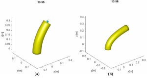
From the screen shots of the animation and the simulation results in Fig. 8.14(c), neither the simulation nor the animation got cracked. Using ROM can perfectly solve the separating segment problem and meanwhile the “fake” animation for EBR is probably caused by the limitation of animation function itself (the tubeplot function), which cannot cope with elongation situation. So maybe in the future, when dealing with large shear force or input, we can try to use ROM to avoid such issues.
8.3 Impact and Contact Dynamics
The impact and contact dynamics are becoming popular topics in the field of soft robotics in recent years with the increasing opportunities for the human and robots to cooperate. Though the soft robots have their own advantages in terms of the material over conventional rigid ones, we still have to put the safety issues to the first priority when designing the mechanical structure and controller to protect human beings from being injured to the maximum extent. In this case, we need to consider about the interaction force between them carefully in advance.
The interaction between human and robot or between the robot and its surrounding environment denotes the primitive meaning of the interaction (contact and impact in this chapter) rather than the more fancy concept of touchable control. And there is a common misunderstanding that impact problem is usually deemed to be identical to contact, actually they are distinct from each other in nature, impact is an instantaneous process which could be happened just in several milliseconds, if we are going to establish an elaborate model, we have to consider about the deformation during this process, if there exists energy loss, if so, how to identify the restitution coefficient? And we also need to apply conservation of momentum if rebounding happens. Instead of making the modelling so complicated, we are going to start from the simplest case, we assume that the time span for this process is so short that any deformation can be ignored and there is no rebounding or energy loss.
To learn how to model system with contact/impact force, firstly we have to state all the assumptions we make, and to make the process much easier to understand, we treat it as “assembly” in the production line, which can be divided into three main sections: from rigid robot to soft robot, human-robot interaction and collaboration assembly and robot-environment impact/contact assembly. The main assumptions are shown as follows:
(1). From rigid robot to soft robot
• The model was set up based on the piecewise constant curvature theory, which means that the deformation will not affect the length of each segment of SRA;
(2). Human-robot interaction/collaboration force modeling
• The inertia tensor has very little influence on the interaction force, which can be ignored;
(3). Robot-environment impact/contact force modeling
Impact Stage:
• The impact process is instantaneous;
• There is no rebounding or slipping between the robot arm and the environment (grasped object) during impact;
• The external applied force can be represented by impulses during impact;
• The impulse forces may result in an instantaneous change in the velocities of robot arm, but no instantaneous change in their configuration (displacement or deformation).
Contact Stage:
• The contact surface is deemed to be a flat surface.
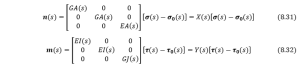
8.3.1 General way to derive the force from EOMs
(1). From rigid robot to soft robot
The canonical format of the governing equation of rigid robot motion for the simplest case can be directly used on soft robots if we temporarily ignore its compliance part resulting in

where the subscript denotes soft robot,  is the mass/inertia matrix,
  is the Centrifugal-Coriolis matrix,
  is the vector of gravitational forces and
  is the vector of robot joint torques or forces, which can be rewritten in another way,

However, for soft robots, apparently Eqn. (8.38) is not sufficient to depict its compliance. Thereby two additional terms, namely, stiffness and damping matrices, should be added to the original model to represent the specification of soft material. If we assume the torsional stiffness of each robot arm link as  and
and  , and the damping coefficients for twist and bending motion are
  and
and  respectively, their potential energy for each part should be as follows,

If we bring Eqn. (8.40) and (8.41) into Lagrange’s Equation, we can obtain the governing equation for the first step as follows,

where the stiffness matrix  and the damping matrix
  . If the model is established using CC, we have to strictly follow the format in Eqn. (8.42), for EBA, EBR and ROM, we are going to derive the motion equations using TMT method [10], which is a more efficient way especially for simulation.
(2). Human-robot Interaction/Collaboration Force Assembly
If we consider the interaction force between human and soft robot is in the form of force, the motion equation below should comply with most conditions if we assume the interaction is a mass-spring-damper system,
![]()
where the generalized interaction force for each joint is  and
and ![]() , in which the subscript
, in which the subscript  stands for human, for joint of SRA,
  is the damping matrix of human body,
  is the stiffness matrix of human body,
  and are the human motion intention (or actual position) and position vector of the soft robot base respectively.
Note: In most papers, it is the end effector of the robot arm that has direct contact with human body, in this case we have to transform the variables under the inertia frame into those under the local frame of each joint/link by  where
where  is the equivalent Jacobian matrix . But in our model, human body is tied with the base of SRA, the task space is to detect and interact with the environment, we can make the transformation in a similar way.
To sum up, the motion equation for this step will become
![]()
(3). Robot-environment Impact/Contact Force Assembly
When a human equipped with the SRA is walking freely without any potential tendency to fall down, the governing equation of the whole system will remain the same as Eq. (8.40); if the tendency was detected (the specific strategies for recognizing falling down has not been determined yet), the “protection mode” will be triggered, the actuators in SRA will begin to work to let the arm grasp some firm objects nearby so that falling will be avoided, and Eq. (8.40) still complies with this process.
However, when the SRA collides with the environment, the dynamics of the system will be switched to another mode, the contact mode. And the contact stage can also be classified into impact and contact (hold) modes. The logic inside can be organized in the way that based on Assumption 4 for this section, we can set a very small default tolerance which can be seen as zero and be compared with the position variation of the impact point within a single sampling time, if , it is deemed that collision occurs, from the next sampling time, the motion equation will be shifted to contact mode.
Stage 1: Impact
Firstly, for the impact stage, the dynamics can be deducted by Lagrange method as follows based on Eq. (8.40),

where  denotes the vector of external forces (actually impulse within a very small time span) acting on the robot joint due to impact/impulse between SRA and the environment. If we use the subscript
  to present the collision point impact stage and
  to represent joint of SRA, for the superscripts + and – are instants after and before impact, according to conservation of momentum,
![]()
where  and
and  .
.
As the velocity just before the impact is determined from the purely actuated stage (non-impact) and meanwhile the impact is much more likely to happen on other positions rather than the joints, we have to use analytical Jacobian to calculate the equivalent force/torque exerted on each joint by ![f_{IJ}=\delta\ M_{IJ}=J_A^T\left(q\right)f_{IC}=J_H^T\left(q\right)\left[\begin{matrix}I&0\\0&R^{-1}\\\end{matrix}\right]f_{IC}](https://opentextbooks.clemson.edu/app/uploads/quicklatex/quicklatex.com-73d1201a6a6338ad770606c5bc5ace33_l3.png "Rendered by QuickLaTeX.com") , where
, where ![J_A\left(q\right)=\left[\begin{matrix}I&0\\0&R^{-1}\\\end{matrix}\right]J_H\left(q\right)](https://opentextbooks.clemson.edu/app/uploads/quicklatex/quicklatex.com-e35ee8696f1d02630d1f9a7e3746d5bb_l3.png "Rendered by QuickLaTeX.com") is the analytical Jacobian matrix,
is the analytical Jacobian matrix,  and
and  denote the impact force exerted on the contact point and joint respectively. We can also define
  by the status of the base
  and their transformation (or rotation) matrix
  as follows:

And then we can apply the principle of virtual work and let denote the position of contact point, we will obtain
![]()
where  .
.
Next, according to assumption 2 in the impact stage aforementioned, there is no rebounding or slipping between the robot arm and the environment , we have

Combining Eqn. (8.46), (8.47), (8.48) and (8.49), we can derive

where ![]() and
and ![]() .
.
Thus the computed impact force acting on the contact point will be

Therefore the motion equation for the impact process should be

Stage 2: Contact
As all the external forces acting on the SRA obey the same rule in terms of the formatting in the motion equation, so as the contact force, and it is exerted on the end-effector of the SRA, we assume the Jacobian matrix mapping from task space to configuration space for this stage is  , where the subscript E stands for environment. The governing equation will be:

where  is the contact force at end-effector. Then the force can be estimated by deformation and geometry factor of SRA (assuming the outer radius of the chamber is and the deformation is
  ),
),

Therefore, the area of the contact surface can be calculated by

According to the definition of stress, we have

where is the Young’s Modulus of elasticity and  is a dimensionless and being negative if stress is owing to compression,
  .
.

where ![]() ,
, ![]() . Then combining Eqn. (8.54), (8.55), (8.56) and (8.58) results in:
. Then combining Eqn. (8.54), (8.55), (8.56) and (8.58) results in:

(4). Summary
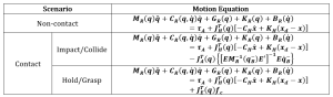
Given the information above, the whole process can be summarized in the table below.
Table 8.2 The summarized motion equations for different scenarios
8.3.2 Other methods about modelling contact force
Sometimes, when the shape of contact surface is not so complex, we can model the contact force as a spring [11] as follows.
(1). Spring-dashpot model
![]()
(2). Hertz’s model
![]()
where  and are constants depending on material and geometry properties and computed by using elastostatic theory.
(3). Non-linear damping
![]()
where it is standard to set  and
and  . For identifying
  and , the relationship can be expressed by the coefficient of restitution as follows,

Summary
As a new star in research area, soft robotics is gradually becoming a comprehensive subject, which is a combination of dynamics, manufacturing, material, control, computer science and even medical and so on. With the maturity of machine learning and deep learning, more flexible control strategies can be applied onto soft robots. Nevertheless, those strategies are more like “black box” to us and largely rely on experimental data training, this makes them hard to be multiple-task-oriented. Therefore, model-based control will still be the main stream in this area, and since the modern control theory is on basis of state space, it is necessary for related researchers to learn about the modeling theories and principles.
This chapter started from introducing some basic prototypes of soft robot manipulators in terms of their driven approaches, cable driven, tendon driven and pneumatic actuated soft robots. The material characteristic of soft robots makes them have better compliance performance than rigid ones congenitally. To reflect the uniqueness of soft robots’ compliance, a simple mass-spring-damper modeling was first proposed, however, due to its inaccuracy of simulation and limitations of assumptions made, three classic types of modeling methods, namely Piecewise Constant/Variable Curvature (PCC/VC) modeling, Euler Bernoulli Beam Theory and Cosserat Rod Theory were introduced to adapt to different application scenarios.
PCC modeling is more suitable for small bending angles or more stiff material, when exerted with a large external or actuation force, the error between simulation results and reality will become larger and larger. VC is an updated version of PCC, which is applicable for soft manipulators with multiple segments, but if the number of segments is large enough or the manipulator needs to be seen as a continuum, the computation cost and efficiency will decrease sharply. Then given this situation, the rest two modeling methods mapping the relationship between the force applied and the manipulator’s space configuration were demonstrated. Euler Bernoulli Beam Theory can be seen as a subset of Cosserat Rod Theory, though both of them are suitable for 3D problem modeling, the former one is better at solving single bending direction problems in the 3D space since we do not consider too much about the twist torque (if we do need to model complex motion with this method, we have to add secondary assumption, i.e., the twist torque will not affect the position of neutral line). On the contrary, Cosserat Rod Theory can perfectly tackle all the issues state previously when doing simulation, but it is hard to realize real time control. Thus when choosing a proper method for modeling, we have to combine it with the actual situation and make a trade-off between computation cost for simulation and control reliability.
Because we have talked a lot about the modeling methods related to external force/torque, meanwhile the collaboration and interaction between human and robots is becoming an even more popular topic, we discussed the motion equation assembly process for different scenarios, with external force/torque exerted on the end effector only and with both the force/torque on the end effector and contact/impact force at an arbitrary position on the manipulator’s body. Understanding this chapter will be beneficial to doing research and study more complicated modeling and control.
Simulation Code & Results
Simulation is always the most efficient and straightforward way to evaluate the modeling assumptions and foundations. But sometimes even the modeling is correct, the simulation still could go failure or get cracked (which means the simulation results get too far away from our expectation) due to inappropriate settings, in our case, it could be too large external load or pressure. Apart from this, without consider deflection factor, all the motion equations should be in the second-order level, and the computers use different logic when solving these differential equations, unlike our human using Newton Leibniz’s integration method, they choose to use numerical integration method, the results can be affected by the step size, tolerance value and so on. And since lots of packages have their own build-in ODE solvers, to guarantee a relatively reasonable simulation result, understanding the mechanism of ODE solvers is important.
So this section will be divided into two main parts: understanding of ODE solvers via a simple SRA simulation and the definition of stiff system, the usage of TMTDyn simulation package and some related simulation results.
Understanding of ODE Solvers
(1). A simple simulation of a falling ball attached with SRA
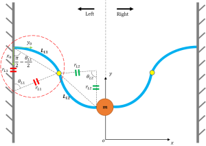
Firstly for our simple simulation, we set a scenario that we have a ball with mass  , which is attached by two identical SRAs, and the end effectors of the two SRAs are tightly fixed on the wall which can be seen in Fig. 8.13 (no sliding). And we assume that the ball is released from an arbitrary position between the two walls without any other external force inputs. And all the other assumptions can be seen below as well.
Created by Yalun Jiang
1). Assumptions
- The model of SRA is set up based on the piecewise constant curvature (PCC) theory;
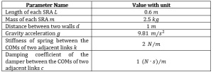
- As it is a 2D problem, we only have to consider the stiffness and damping of bending rather than twisting (the specific values for the parameters were referred from Chase’s dissertation);
- The only external force is gravitational force acting on the ball for stage 1;
- The two end-effectors are attached to two fixed points (same altitude) throughout the whole falling process;
- The curve at the ends connected with the wall and the ball is always tangential to the horizontal surface;
- We treat each SRA segment as three links, two for revolute and one for prismatic;
- In the transformation matrix, the z axis is always deemed to be along the axle of revolute or the prismatic direction.
2). EOM Derivation
Using the similar process discussed in Section 8.2.2, the equations of motion can be separated by two parts, the left SRA and the right one, which can be simply summarized as follows,
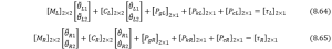
where  and are the inertia matrices for left and right SRAs respectively,
  and are Coriolis Centripetal matrices, and for the potential energy part, it can be divided into three parts due to the specification of this model, namely gravity (
 and
and  ), spring stiffness (
 and
and  ) and damping (
 and
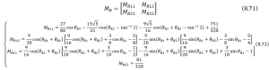
and  ), their specific expressions can be seen below. From the coding experience of “falling SRA” project first version (using PCC theory). The code is able to visualize the specific expression of each matrix for each time step, and simplify them as much as possible. However, Mathematica has a superiority over MATLAB in terms of symbolic variable calculation, so according to the complexity of each expression after the first processing of MATLAB, the complexity of inertia matrices is acceptable, the rest was simplified for the second time by Mathematica, for the brevity of the expressions, some of the parameters have been assigned with specific values at the start, which can be seen below.
Table 8.3 Parameters of SRA properties assigned
– Inertia matrix ( )
)

Each element in the matrix is so complex, thus for the following matrices, we are going to pick them out individually as follows.

For the right arm, we have
– Coriolis-centrifugal matrix ()

where each element in the matrix is shown as follows,
– Potential energy due to gravity

– Potential energy due to “spring” stiffness
– Potential energy due to damping

3). Simulation Results
The simulation package is open source on GitHub: https://github.com/TheThigh/WEMADE. To start the simulation (we assume the motion for the left and right arms are symmetric about the central line of the two walls), the initial conditions and other parameters were set as follows,
Table 8.4 The parameter setting to trigger the simulation

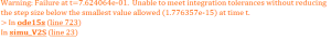
The simulation solved by ode15 function can run successfully without any errors, the only limitation was that there are a few lines of warnings in the command window which can be seen in the figure below,
Created by Yalun Jiang
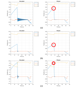
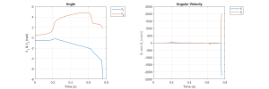
And the simulation results are shown in the figure as follows, the figure on the left is the angle change, and the right one is the angular velocity; the results for the angular velocities could vary quite a lot with the increasing of the time step, the trend of angle change remained almost the same for different time step settings.
Created by Yalun Jiang
Moreover, the simulation time didn’t comply with the time span we have set for triggering the simulation, the simulation aborted at around 0.8 s, which is exactly as the warning told us, so according to the feedback in command window, I have tried to change the relative and absolute tolerances, the simulation still stopped at 0.7624064 s. After that I looked up some resources in MATLAB Community, somebody said it might be due to the singularity problems of the matrices, but I have recorded the eigenvalues of the inertia matrix for each time step, they are all positive values. So a brief conclusion can be drawn that, sometimes it is not our fault that leads to a failed simulation, it is the setting that we have to pay more attention. That’s the reason why we have to learn how to choose proper ODE solver starting from stiff system in the subsequent sections.
(2). Basic concepts of stiff equations
As the simulation tools like MATLAB/Simulink solve ODEs using numerical integration method which is quite different from the analytical/exact solutions computed manually, clearly utilizing different ODE solvers might lead to significant different solutions and simulation results, and the selection of ODE solver largely depends on whether the system is stiff or not, thereby, it’s crucial important for us to understand the concept of stiff systems.
A stiff system can be composed of multiple differential equations, so we probably need to start from a single differential equation to learn about what is a stiff equation firstly. Generally, if the solution of a differential equation (worked out by numerical integration) is quite unstable unless a pretty small step size was chosen, the equation is so-called stiff. Or we can express it in a more understandable way, if the motion of a certain object can be written into a set of governing equations, there maybe exist several subsystems that have significant variation rate, this process or motion can be deemed to be “stiff”.
If it is still too hard to understand this concept, the following examples might better demonstrate it. Consider we have two differential equations as follows,

The exact solutions of them are  and
and  respectively, however, these are done manually, it will be another story for numerical method, like Euler’s method. According to the basic principles of that method, we have
![]()
where  and
and  stand for the estimated value of
  and
and  steps of iteration of
  ,
,  is the step size can be selected according to our needs and
  can be seen as a simple expression of the differentiation
  , which is a function of both and sampling time
  . If we set the initial conditions for both the Eqn. (8.87) and (8.88) are
  , and the test values for are 0.00001, , respectively, the simulation results in Simulink will be shown as follows,
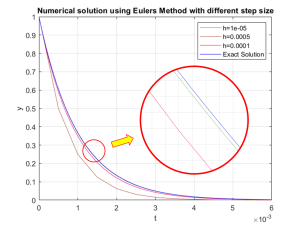
 with different step size.
Created by Yalun Jiang
However, when the step size is relatively large, the computed results will not be accurate anymore, and moreover, with the increasing of the simulation time, the system which should converge now becomes unstable, the proof is shown as follows,
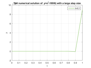
Created by Yalun Jiang
Since smaller step size will lead to more accurate solution, we will try what happens for slow decay system  in Eqn. (8.88) with larger step size,
  respectively. From the plot below, we can see that even with pretty large step size compared with that used in
  , the difference between the numerical and exact solutions can be as minor as 0.002, which is acceptable.
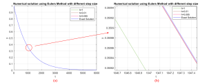 (a) full scale solution in the simulation time. (b) partial enlarged drawing of circled position in (a).
Created by Yalun Jiang
Again, to testify the influence of step size on the accuracy of the computed solution, in this turn, a very small step size 0.00001 was chosen for simulation, the results will be displayed below.
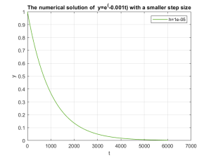
 with an even smaller step size.
Created by Yalun Jiang
From the simulation results above, we can conclude that smaller step size will only make the computed solution of ODE more accurate sacrificing the computation time, it took around 3 mins for my PC with 32 GB memory to simulate it. And we find that for fast decay or convergence system (with large  value, which is the coefficient before in Eqn. (8.87)), the change is so large within a tiny time span, numerical solution with large step size will not reflect the real results, which means that the equation is stiff.
(3). Basic concepts about stiff systems
Slightly different from the definition of stiff ODE, a stiff system should be composed of at least one equation that has very fast and very slow variation term (the value) simultaneously, if we still use the example and in the previous part, now we can forge a new expression

And we find that if we set the step size as  , the numerical solution for the fast variation part
  will be ignored, when the step size is chosen to be smaller and smaller, the characteristic of the equation will be reflected. In the Eqn. (8.90), we can define that
  ,
,  , a new concept, stiffness ratio can be brought in as follows,

And we find the ratio is very large, so the system is very stiff. And then another question might emerge, how could we know if a system is stiff or not, is there any rubric for the stiffness ratio? Before explaining this, let us review the general solution for a second order ODE,

The stiffness ratio only has practical meaning when the system has two different real roots (for a second order system), it is sufficient for analysing most of the dynamics. For higher order systems, they will have more characteristic roots or eigenvalues, to express the stiffness ratio in a more general and rigorous way, we have

That is because only the real part of the roots domains the decay or growth rate. And now we consider an even more complex dynamic system with multiple state variables  ,
,  , …,
, …,  , we will have the following governing equations in the matrix format,
And the exact solutions of the state variables  will be in the form of Eqn. (8.92), in this case, there will be a stiffness ratio for each variable, compare each of them and then we can determine if the system is stiff or not. However, it can be extremely hard to obtain the exact solution of such system as the stiffness ratio varies with time continuously, the best way for doing simulation about system alike is to follow the suggestions for solving ODE (in MATLAB/Simulink), try ode45 first, because it can handle most of the problems, if it doesn’t work, we can move on to try other implicit solvers, the specific information about ODE solvers will be introduced in Section (4).
Now we turn back to discuss the rubric to judge whether a system is stiff or not. According to the theory proposed by Lambert in 1973, a system can be classified as follows,

If the ratio is greater than 1000 for a system, it is recommended that a smaller step size should be applied to guarantee the precision of the numerical solution.
(4). Specifications of different ODE solvers in MATLAB/Simulink
Since we have spent a huge paragraph to demonstrate the definitions of stiff differential equations and systems, we know that the step size largely influences the accuracy of the numerical solution for a stiff system, meanwhile it’s hard to determine if a complex system is stiff or not because the stiffness ratio changes with time, which is super dynamic, in this case, selection of proper ODE solver is extremely important for precise simulation results.
In general, the ODE solvers can be classified by explicit and implicit ones, the explicit ones are good at coping with non-stiff system; on the contrary, the explicit solvers are excel in dealing with stiff systems, which have the letter s,t or tb after the number of order, like ode 15s, ode 23t. For a relatively simple model, we can follow the steps to choose the ODE solver.
However, when a model becomes more complex, we need to evaluate each solver.
1). Fixed step ODE solvers
Theoretically if the step size was set to be small enough, any model can be simulated accurately, the only drawback is the computation cost. But it doesn’t mean that it is of no use for fixed step solvers. For code generation used in embedded platform, fixed step solver must be used. And compared with variable step solvers, the fixed ones do not have to compute the step size for each step individually, which will take up additional memory of the computer, usually we need to do some tests using other solvers and analysis to confirm final step size on basis of making a balance between simulation precision and computation cost. The procedure to determine the step size will be shown as follows,
- Step 1: Select at least three variable ODE solvers to get a rough baseline result;
- Step 2: Select one of them as standard result which can be used to compared with the fixed step solution;
- Step 3: Confirm an acceptable tolerance and step size;
- Step 4: Perform the fixed step simulation and compare with the standard result you choose for the variable step solver in Step 2;
- Step 5: Repeat the Step 3 and Step 4 until we have found the result of fixed step is within the tolerance, and confirm the maximum step size.
2). Variable Step ODE Solvers (most frequently used)
- Explicit solvers
ode 45: First choice for most problems with medium accuracy, if the computation is slow, we should try to use some implicit solvers because the system might be stiff.
ode 23: If the error tolerance is cruder than ode 45, and the system is slightly stiff, the efficiency can be improved using this solver, but the accuracy might be a little lower.
ode 113: Multiple step solver, if the error tolerance rule is strict according to our simulation needs, it is recommended to use this one, the accuracy can be variable from low to high.
- Implicit solvers
ode 15s: Multiple step solver, it can handle stiff system, though with the increasing of orders, the accuracy will be improved, the stability will be decreased; if the system is stiff and stable, the highest order should be set to 2 or use ode 23s instead. (accuracy: low to medium)
ode 23s: Single step solver, applicable for moderate error tolerance, second choice for solving stiff system problems.
ode 23t & ode 23tb: Use trapezoid rule to realize, the accuracy is low.
2. Simulation Using TMTDyn Package
The TMTDyn Simulation Package is also an open source which is available on GitHub: https://github.com/smhadisadati/TMTDyn. Though it was not GUI oriented, we can still master it quickly as most variables can be told by their names. This package is friendly to users that are not familiar with dynamics or that do not want to spend so much time on modeling. This section will cover some entrance level guidance of its usage and some simulation results.
(1). Package Operating Instructions
The results (shown in Fig. 8.20) are composed of the simulation results (solid line) and the real experimental data (dashed line), the package is proved to be reliable especially for short appendage. When running the simulation with our own settings, the real experimental data will still be kept on the plot, which is actually of no use of us, sometimes it will cause confusion to the audience who is not familiar with the package. So the first step is to block these data.
Created by Yalun Jiang
The related function is stored in the path eom\post_proc.m, we just need to comment out all the experimental data (par.tip_exp) plot sentences, after doing this, the effect is shown as below.
Created by Yalun Jiang
You may get familiar with the package by changing the geometry factors in the m files with the name from exp1 to exp6 in v6_Latest_Version_Examples, the 6 examples represent different modelling methods mentioned in [10], for more details you can either check the YouTube video provided by Dr. Sadati (https://www.youtube.com/watch?v=nQUO1ugRiK0&list=LL&index=2&t=4230s), or visit https://github.com/TheThigh/SRA/tree/main/Weekly_Report for more comments, debugging and simulation results about the package. As stated previously, the first thing we recommend might be duplicate the simulation done in [10], then you can adjust the parameters (at the very beginning part of the code) to fit with your own project or needs. The configuration of the manipulator in the package is slightly different from what we usually see, it has two pneumatic chambers to control a bending direction, if you have only one chamber to control one bending direction, you have to adjust the offset angle phi_o to zero. And if you are going to do simulation on exactly the same manipulator, you may change the highlighted word “full_system” to “no” in Fig. 8.22 after the first time you run the code so that the EOMs (it will be stored in eom file and not be over written) will not be derived again and again to improve the efficiency of simulation.
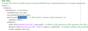
Created by Yalun Jiang
If you want to do simulation with multiple manipulators, please check the link https://github.com/TheThigh/TMTDyn_Multi_Arm_Simu, which is the modified version, and accordingly we also need to edit your input condition for each manipulator in data_editor.m.
(2). Simulation Results
1). The influence of manipulator parameters (length) on simulation results
As our physical SRA has two links, the length of each is about 30 cm, the total length should be around 60 cm, which is about 15 times by the length of the manipulator stated in the Sadati’s paper [10], and the package seemed not to have a good performance for very long manipulator, it’s necessary for us to do more tests.
The first control test group was to increase the length of the manipulator from 100 mm to 200 mm, since I found that when the length was set to be 150 mm, the animation and the position of the tip seemed not good, here comes the second test group to verify the influence of number of links/segments on the simulation results, the number was set to be 2, 3 and 4 respectively; and for the third one, since issue began to occur for length equal to 150 mm, I decided to modify the outer radius of the manipulator to see if the animation is normal. And all the results are shown below.
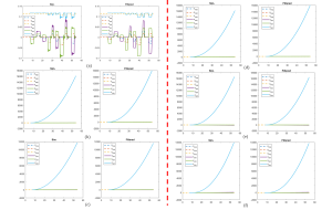
 =100 mm, (b)
  =150 mm, (c)
  =200 mm; (d) =2, (e) =3, (d) =4.
Created by Yalun Jiang
From the simulation results above, we can clearly find that for the test of increasing length for the number of links with 2 (on the left side isolated by the red dash line in the middle), the position of the tip began to be abnormal when the length is greater than 150 mm, and the unit for y axis for these plots are all in meter, so obviously the results are not rational. Then I thought if the number of links will affect the accuracy and results of the simulation entirely, to this end, we found that indeed the increasing number of links will improve the accuracy (from about 16000 m max to about 14000 m max) sacrificing a lot of computation time, however it did not have any decisive effect on the final trend.
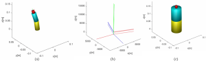
 s (a)
s (a)  =100 mm,
  =12.5 mm, (b) =150 mm, =12.5 mm, (c) =150 mm, =30 mm.
Created by Yalun Jiang
And to investigate what other parameters of the manipulator determine the simulation results, we decided to change the outer radius of the manipulator for the specific length whose simulation results (position of the tip) seemed quite abnormal, from the figure above, it’s not difficult to draw that except for the length of the manipulator, if we keep all the other parameter the same, the results went crack for length 150 mm, however, when we modified the outer radius of it from 12.5mm to 30 mm, the simulation animation went back into control again even though the position variation was not so obvious, partially it was owing to the enlarged stiffness of it by increasing the radius (more material infilled).
So far we can draw a very rough conclusion based on the simulation results from the two control test groups, which will be listed as follows,
- The length of the manipulator will affect the simulation results largely, however, it is not the limitation or fault of the package itself to cause this kind of failure, controlling the ration between the length and outer radius of the manipulator will lead to a good simulation result in most cases;
- The number of links/segments will affect the accuracy of simulation, the basic principle behind is like FEM, but when it exceeds a certain value, the improvement will not be so apparent any more, it will become meaningless to sacrifice so much computation efficiency then;
- This one is more like a hypothesis rather than a conclusion. The main reason for the failure of most simulations mentioned above can be owing to the geometry factor of the manipulator itself, the manipulators in all the failed cases were deemed to be very “thin”, they would easily fall down on the ground even subjected to a minor disturbance at the equilibrium point. The additional test by increasing the outer radius of the manipulator can successfully support this standing, when the radius is becoming greater and greater, it will gradually become a “cylinder” from “stick”, it will be stronger to support its own gravity and easier to swing back to the equilibrium point after the force/torque acting on the tip is eliminated. Another way to testify it is to enlarge the pressure input in all three chambers for the very “thin” manipulators, and see if they can acquire better simulation results.
2). The influence of pressure change in the chamber on simulation results
According to the hypothesis proposed previously, if we increase the pressure in certain chamber(s), and the SRA would swing back, it can be proved that the length setting of the model is not the limitation of the package. However, before doing that we have to make sure the meaning of data of each column in “NoLoad.mat” file, from the comments in the “sample_exp_data.m” file for the input mode 1, we have the following definitions.
Table 8.5 The definitions of the inputs for mode 1

Still using the control test method, we find that the names of the columns comply with some basic principles, for example, the prefix of the column 2 to 4 is Pres, which probably means the pressure supply for each pneumatic chamber for the SRA (needs to be further confirmed), to this end, our secondary experiment can be classified into 6 groups, the original group, zero elements (input) for column 2 to 4, zero elements (input) for 5 to 7, from 8 to 11, from 12 to 14 and from 15 to 18 respectively. My plan was to set all the elements of the columns mentioned for each test group as zero, on one hand we can figure out which parameters are the real inputs to trigger the simulation; on the other hand, we can check if the pressure supply domains the dynamics of the SRA by multiplying it in the subsequent tests.
The simulation results for the six tests have been showcased as follows, in which the dash lines represent the experimental results and the solid lines stand for simulation results, except for (b), the simulation results are exactly the same, the most likely reason is the input changed in group (b) is the real input of the simulation, which is pressure; for the rest figures, the experimental results vary for each one, which seemed pretty weird because we have just confirmed the pressure is the only input and real experiment data would not be affected by simulation input.
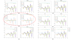
Created by Yalun Jiang
To find the reason behind, we probably need to check the specific input in the next figure below. Still in the figure (b), we can clearly find that no matter for the pressure of each chamber, the force acting on the tip or the torque on the tip, they are all zero, but the position of the tip is not always zero, so there is only one chance that it should be the position record of the real experiment. And the position of the tip varies with the same principle for the first four figures, in (e) and (f), the position performed with a totally different manner, the summation of (e) and (f) coincides with the other four, maybe there are some system offsets or filters in the last seven columns of input data, we can study it in the future, as it is not the main focus of our research right now.
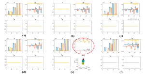
Created by Yalun Jiang
Practice Problems
- Please state at least two advantages and disadvantages for modelling method PCC and Cosserat Rod Theory.
- Use the example in Fig. 8.4, we assume that there is a ball (the geometry factor can be ignored) with mass attached with the end effector of the arm. The arm was fixed on the wall, it has two segments with equal length , which will not change with the change of the bending angle
 . To mimic the compliance of soft robot manipulator,linear damper (
 ) and spring () are added that connect the COMs of the two segments. Please derive the motion equation(s) of the system for an arbitrary bending angle .
 - Consider a soft robot arm with two segments, we assume the twist angles of two segments are
 and
and  , the bending angles are and respectively. Derive the motion equation(s) of the system using VC theory, the curvature and mass of two segments are , and
  ,
,  , the COM of both segments are deemed to be in the geometry center, this time we need include the angular velocities.
References
[1] Watts. “Swallowtail Caterpillar on Fennel Plant.” Flickr, Jul 17, 2017. https://www.flickr.com/photos/watts_photos/35816343066.
[2] Marshall, Jerry. File:Big Sur Snake.JPG, February 19, 2013. https://commons.wikimedia.org/wiki/File:Big_Sur_Snake.JPG.
[3] File:Sea Horse.jpg, July 20, 2018. https://commons.wikimedia.org/wiki/File:Sea_Horse.jpg.
[4] Malhotra, Param. “Soft Robotic Arms for Fall Mitigation: Design, Control and Evaluation.” (2022).
[5] Spong, Mark W., Seth Hutchinson, and Mathukumalli Vidyasagar. Robot modeling and control. Vol. 3. New York: Wiley, 2006.
[6] Wang, Jue, and Alex Chortos. “Control Strategies for Soft Robot Systems.” Advanced Intelligent Systems 4, no. 5 (2022): 2100165. https://doi.org/10.1002/aisy.202100165.
[7] Erochko, Jeffrey. “5.2 The Bernoulli-Euler Beam Theory.” 5.2 The Bernoulli-Euler Beam Theory | Learn About Structures, 2020. https://learnaboutstructures.com/Bernoulli-Euler-Beam-Theory.
[8] Wang, Hesheng, Hang Ni, Jingchuan Wang, and Weidong Chen. “Hybrid vision/force control of soft robot based on a deformation model.” IEEE Transactions on Control Systems Technology 29, no. 2 (2019): 661-671.
[9] Sadati, SM Hadi, S. Elnaz Naghibi, and Mahyar Naraghi. “An automatic algorithm to derive linear vector form of Lagrangian equation of motion with collision and constraint.” Procedia Computer Science 76 (2015): 217-222.
[10] Sadati, SM Hadi, S. Elnaz Naghibi, Ali Shiva, Brendan Michael, Ludovic Renson, Matthew Howard, Caleb D. Rucker et al. “TMTDyn: A Matlab package for modeling and control of hybrid rigid–continuum robots based on discretized lumped systems and reduced-order models.” The International Journal of Robotics Research 40, no. 1 (2021): 296-347.
[11] Gilardi, Gianni, and Inna Sharf. “Literature survey of contact dynamics modelling.” Mechanism and machine theory 37, no. 10 (2002): 1213-1239.
