
3 Force Control of Robots and Applications in Advanced Manufacturing
Rahul Narasimhan
Chapter Outline
3.1 Background
3.1.1 Passive and Active Interaction Control
3.2 Indirect and Direct Force Control
3.2.1 Indirect Force Control
3.2.1.1 Impedance Control
3.2.1.2 Admittance Control
3.2.1.3 Impedance vs Admittance Control
3.2.2 Direct Force Control
3.2.2.1 Hybrid motion/force controller
3.3 Advanced Manufacturing Applications
3.3.1 Impedance Control of a Lower Limb Exoskeleton used for Lifting
3.4 Summary
Simulation
Practice Problems
Reference
3.1 Background
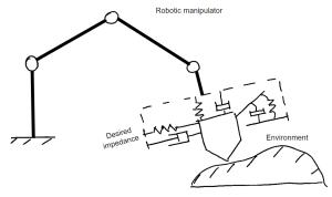
In the recent decade, research with robot force control has been increasing with an increasing number of use cases in medical, occupational, construction, and many other industries. Typically, any task that involves robot interaction with an environment such as polishing, cutting, scraping, pick-and-place, welding, etc. [26] can benefit from the use of different methods of force control strategies (see fig. 3.1). Another field where force control has a major role to play, and potentially have a big impact is physical human robot interaction [1]. This typically involves a robot working in synchronous to the human where the robot measures the motion or forces from human and correspondingly responds to complete a desired task.
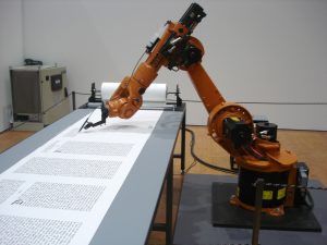
“Roboscribe KUKA Robotics.jpg” by Marc Wathieu is licensed under CC BY 2.0
3.1.1 Passive and Active Interaction Control
Control of the physical interaction is essential to successfully complete tasks involving end-effector of a robot that has to manipulate an object or complete an operation on a medium [10]. There are two types of interaction controls – passive and active interaction controls. In passive interaction control, the trajectory of the end-effector is driven by the interaction forces due to the inherent nature or compliance of the robot (i.e., internally, such as joints, servo, joints, etc.) [10]. An example would be soft robots where such robots are intrinsically designed to have materials and properties that are safer for human interactions. But it lacks flexibility because every specific task might require a special end-effector to be designed and it can also have position and orientation deviations. High contact forces may also because there is no force measurement [10]. In active interaction control, a control system is designed specifically which usually involves measuring contact forces, moments, track the motion and feeding to the controller that can produce the desired action in terms of trajectory or object manipulation (for example see fig. 3.2) [10]. Although they are advantageous compared to the shortcoming with passive interaction control, they are usually slow and expensive to implement [23]. Additional strategies to reduce noise and disturbance may be required where some degree of passive compliance too [10]. Active interaction control can be further grouped into indirect (such as admittance and impedance control) and direct force control strategies (such as hybrid force/motion control). Further details about indirect and direct force controls will be covered in the following sections.

“KUKA Robot Painter Nagyoa Robot Museum.jpg” by theloneconspirator is licensed under CC BY-SA 2.0
3.2 Indirect and Direct Force Control
Based on achieving force control through motion control strategies without needing the explicit need to close the force feedback loop and achieving force control through by explicitly controlling contact forces and moments to close the force feedback loop active interaction control can be categorized as indirect and direct force control.
3.2.1 Indirect Force Control
In principle this strategy does not require direct measurement of contact forces and moments (say using an external force sensor) [10]. Any deviation of end-effector from desired trajectory arising from interaction with the environment can be controlled assuming that the robot is described by an equivalent mass-spring-damper system where the parameters such as stiffness and damping coefficients can be adjusted [11]. It can be further classified as Impedance or Admittance if the robot responds by generating forces (i.e., through joint moment(s) and/or force(s)) or if the robot responds by imposing a deviation from desired trajectory as a result of interaction with the environment.
3.2.1.1 Impedance Control
In principle, the fundamental idea builds from the fact that mechanical impedance is a measure of how a structure resists motion when it is subjected to a force [18]. As described before, using impedance control results in generating forces through joint moment/force(s) based on interaction with the environment described by equation 3.1 where F is the force, Z is the impedance, and v is the velocity.

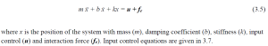
The robotic system is then modeled as an equivalent system with mass, spring, and damper [11]. The one where its parameters such as mass, spring constant, and damping coefficient can be adjusted as required to adapt to the interaction with the environment [8, 9]. For the first part, force and mass relation can be given by Equation (3.2) where m is the mass and a is the acceleration. For a certain force on an object, it accelerates corresponding to the mass of the object. Second part, according to Hooke’s law given by Equation (3.3) where k is the stiffness and x is the displacement, for a certain force on a spring, it displaces corresponding to the stiffness. And for the last part, given by Equation (3.4) where c is the damping coefficient and v is the velocity of the object. The faster the velocity of an object for a given damping coefficient more force is required [25].
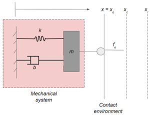
Considering a mechanical system described by Figure 3.3 and 3.4 based on [1],
Created by Rahul Narasimhan Raghuraman based on information from [1]
Created by Rahul Narasimhan Raghuraman based on information from [1]
Here, xe describes position of environment, xr represents the trajectory. Position error is given by difference by x (current position) and the reference (xr) [1].

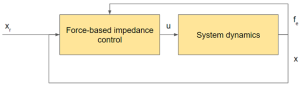
Since the robot is described as a combination of mass, spring and damper, the equation for the desired trajectory is given by Equation (3.7) and Figure 3.5 illustrates an example of an application.

Created by Rahul Narasimhan Raghuraman based on information from [4]
Hence, by controlling the impedance of the robot we can manipulate the behavior of the end-effector depending on the interaction with the environment. For example, we can set very low impedance (or high compliance) and make it act like a very loose spring or we can set the stiffness very high where the robot would only move to the desired position without much oscillation.
3.2.1.2 Admittance Control
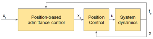
In this type of active interaction controller, the idea is to alter the position sources by adjusting the stiffness in response to the interaction forces by giving deviation from the desired trajectory [4, 13]. In this method there are two loops – (1) inner loop, where the compliant position or velocity is controlled and an (2) outer loop where the target desired impedance is provided, this delivers the commands for compliant reference (see fig. 3.6 for general description)
Created by Rahul Narasimhan Raghuraman based on information from [4]
For a similar example as described before (see Fig. 3.7) but with an additional reference trajectory to use and command the manipulator, xc.
Created by Rahul Narasimhan Raghuraman based on information from [4]
Based on this, the outer admittance filter is described by Equation (3.8) as –

And the inner position control can be expressed using PID (proportional, integral, and derivative) control methods as shown by equation 3.9 [4].

Here, kp and kv are the gains of feedback.
3.2.1.3 Impedance vs Admittance Control
Because of the assumption of force controlled systems and position controlled systems for an impedance (or force-based) controller and admittance (or position/velocity based) controller their stability and performance values may vary. Therefore, some critical points should be considered when deciding the course of action for controlling a robot as described below [4] –
(1) The inner feedback loop (for position) is required for admittance control whereas it is option for impedance control to include an inner feedback loop.
(2) Almost all modern day industrial manipulators are equipped with servo position feedback hence redesigning the inner position loop can be avoided
(3) Instability problems may occur in force based control as a result of stiff impedance behavior. For a softer environment stiffness of end effector should be stiffer and vice versa. In comparison, position based control can implement stiff behavior better than compliant behavior, meaning that it can be better suited to use admittance control for interaction with a softer or compliant environment.
(4) Host system’s back drivability and friction can also play a role and it might affect stability and performance for an impedance control whereas for admittance the performance depends on inner loop control and quality of force sensor recordings.
3.2.2 Direct Force Control
Direct force control uses explicit control based on the interaction with environment and based on the interaction and contact force, the force at joint(s) of the robot can be controlled so as to complete the task. For example, consider a 1 degree of freedom linear robot as shown below in Figure 3.8 where it is position controlled [20]. Our aim is to control contact force (f) between end-effector of robot and the environment (fref, which can be assumed to be constant).

Created by Rahul Narasimhan Raghuraman based on information from [20]
For such a scenario we can use a PD (Proportional, Derivative) control method. In this system a force sensor measures the contact force between robot’s end-effector and the environment (wall). Starting at sensed force of 0 at the beginning and causing an error in force > 0 therefore causing position error > 0, causing the robot to move right towards the wall.
But in general, the task complexity is much higher where we may have to provide a model to specify desired motion and contact force/moment corresponding to the constraints imparted by the environment on the robot. Typical strategy to work with such type of control system is hybrid force/motion control that generates motion in directions that are unconstrained and force/moment in task direction that are constrained [21].
3.2.2.1 Hybrid motion/force control
Oftentimes robotic manipulators are constrained that limit their motion in the environment in which they desire to complete a task [19]. These are defined as natural constraints and when they to perform a specific task more constraints are given which are called artificial constraints [21]. With hybrid motion/force control the basic idea is to move the joints freely in unconstrained directions while controlling torque/force in the constrained direction due to interaction with the environment as a result of contact [21].
The basic model can be given by the concept that connects constraints for doing a task that requires force feedback to control design. {C} is the constraint coordinate system and transformation form {C} is given such that for controlling one manipulator joint involves every dimension in {C} [21]:

where, qi is the ith joint position of manipulator, is the inverse kinematic function and xj is the position of jth degree of freedom in {C}.
In hybrid control, each joint with actuator drive signal represents that particular joint’s simultaneous contribution to satisfy position/force constraint [21]. The ith joint’s actuator control signal N components that corresponds one for each force and position controlled dof in {C}.

Where, is the torque applied by actuator i, denotes position error in jth degrees of freedom of {C}, denotes force error in jth degrees of freedom of {C}, denotes the force compensation function for input j and output i, denotes position compensation function for input j and output i, sj denotes compliant selection vector’s component.
S is a compliance selection vector. It’s a binary tuple, it specifies the degrees of freedom in {C} that are under positon control and that are under force control (sj = 1). Still the number of active control loops stay N. A compliance selection matrix is also defined as diag(S):

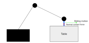
Figure 3.10 describes the idea of a hybrid controller system. Also , the sensory signals as shown in the figure 3.10, should be transformed from coordinate system of transducer, {H} for force and {q} implying position to {C} before errors:

where, X denotes manipulator hand’s position, denotes the kinematic transform from {q} to {C} and F denotes the force acting on manipulator hand.
denotes force transformation matrix from {H} to {C} and denotes rotation matric from {H} to {C}. With this the error signals in position and force by applying equations 3.9 and 3.10:

An example setup shown in Figure 3.10 can be used to demonstrate the principle of hybrid motion/force control (osrobotics.org). Imagine a table and a multi DOF robot that comes in contact with the surface and then proceeds to have a sliding motion. These types of tasks are very common in grinding, polishing kind of jobs in industries [26]. Here the contact force is being controlled in the Z direction while keeping the motion in X direction using a PD controller and a force sensor attached to the end-effector of the robot.
Created by Rahul Narasimhan Raghuraman based on information from [20]
3.3 Advanced Manufacturing Applications
Work-related musculoskeletal disorders (WMSDs) are caused by cumulative trauma affecting soft tissues. Being highly prevalent in manual material handling (MMH) tasks in manufacturing industries, back injuries alone account for 39% of all WMSDs, accentuated by cumulative trauma from repetitive lifting and holding non-neutral postures [6].
Wearable assistive devices such as exoskeletons are being pursued as promising solutions for MMH. Exoskeleton is a wearable technology of large-scale interest in the occupational area, developed to support users while performing work tasks and reducing physical workload by providing external force in body segments [14, 2, 22] They are promising solutions to reduce WMSDs. Being highly prevalent in manual material handling (MMH) tasks, back injuries alone account for 39% of all WMSDs, accentuated by cumulative trauma from repetitive lifting and holding non-neutral postures [5,6]. The National Safety Council recently reported an estimated $164 billion in expenditure due to such work-related injuries [24]
According to the force generation mechanism, the exoskeletons are generally classified into active or passive types [7]. A passive exoskeleton is more present commercially in the occupational context. It is composed of mechanical springs, or dampers to support the human motion, and according to the exoskeleton design, the device will accumulate energy by the motion of the user and generate torque to the target joint to be supported [3, 14, 2]. On the other hand, active exoskeletons may have one or more actuators that can augment the power of user by actuation biomechanical joints such as the hip, knee, ankle, etc [22]. The actuators may be pneumatic, electric motors or hydraulic. There are promising outcomes in terms of reduction in muscle activity, perceived discomfort , energy expenditure [12,15,16,17]. An example of a prototype assistive robotic limb by cyberdyne is shown in figure 3.11.

“Hybrid Assistive Limb, CYBERDYNE.jpg” by katsumotoy is licensed under CC BY 2.0
Mostly impedance or admittance control techniques are used to get a compliant exoskeleton device because it involves a robot-human interaction [13]. With an established use case in manufacturing industry the following section demonstrates lowering and lifting activities supported by an exoskeleton device for reduction in moments at the low back and controlling this action using impedance control.
3.3.1 Impedance Control of a Lower Limb Exoskeleton used for Lifting
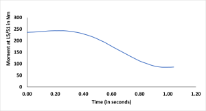
By modeling the human biomechanics for a lifting task we can approximate torque generated by hip muscles. To illustrate a typical lifting task, let us assume a 72.5 kg worker that was required to lift a box from a cart to knuckle height. Using an optoelectronic motion capture system quantitative data were obtained at 120 Hz with markers placed at joint centers of ankle, hip, shoulder, knee, and box. The box mass was assumed to be 25.5 kg. Figure 3.13 below shows a lifting action, the duration of activity is ~1 second and corresponding to this lifting motion, a moment acts at the L5/S1 joint (lower back) as shown in figure 3.14.

Created by Rahul Narasimhan Raghuraman based on [27]
Created by Rahul Narasimhan Raghuraman based on [27]
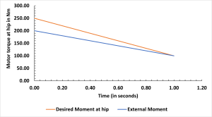
It is assumed that a motor with 25 Nm continuous torque capabilities is used bilaterally on the hip joint on the exoskeleton. An impedance control can be used in this scenario given these characteristics. Based on the moment output for the activity we can approximate an external and desired moment at hip as shown in figure 3.16.
Created by Rahul Narasimhan Raghuraman based on [27]

where, M denotes the moment at hip given by the motors, K denotes the stiffness constant, D denotes the damping coefficient, is the desired position and is the current position, are their corresponding angular velocity parts. It is also assumed that while simulating, the exoskeleton setup has an encoder to record position values.
3.4 Summary
With the increase in the use of robots in various applications with tasks that are increasingly complex choosing an appropriate control strategy is important. In this chapter various force control strategies were introduced. Force control can be implemented by direct or indirect methods by explicit control of force exerted by the robot or by controlling the force indirectly by position/velocity control. With indirect force control, impedance and admittance control methods were used where the robotic system was considered to be an equivalent mass-spring-damper system. Impedance control involved control of the force output based on adjusting the impedance parameters and admittance control involved control of position/velocity output based on adjusting the admittance parameters. With direct force control, an example was described using PD (Proportional-Derivative) algorithm to demonstrate explicit control based on force feedback followed by introduction of hybrid motion/force control method where the robot’s end-effector is directed to move in unconstrained direction while applying force/torque in constrained direction.
Finally, the positive benefits of using powered robotic exoskeleton technologies for manufacturing industries was described. These devices can potentially reduce work related musculoskeletal disorders and improve performance of the workers. An example task was analyzed with given anthropometric and hip joint torque characteristics and impedance control strategy was introduced for completing a lifting activity with an exoskeleton with dual motors attached at hip level.
Simulation
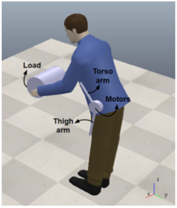
Like introduced in section 3.3.1, a lifting model was simulated using exoskeleton in CoppeliaSim Edu 4.5 (Coppelia Robotics AG, Zurich, Switzerland). Using CoppeliaSim’s library, a male manikin was imported, the characteristics are reported in Table 3.2 [30]. The upperbody is comprised of hands, forearms, upperarms, head and torso and individual body segment’s mass values were calculated like described in Table 3.1. The male manikin used in the software is shown in Figure 3.17 [30] with details about exoskeleton and reference axes.

Created by Rahul Narasimhan Raghuraman using information from [30]
Created by Rahul Narasimhan Raghuraman using [28]
Description of lifting action
- The lifting action takes place starting at a trunk angle of 70 degrees. Trunk angle is defined as the angle of torso w.r.t. the vertical axis.
- Only the trunk is used for the lifting, i.e., stoop only lifting action to simplify model.
- The angle covered is 60 degrees in counterclockwise direction w.r.t. X axis. The final trunk angle is 10 degrees.
Assumptions
- The load, hands, forearms, upperarms, head and torso are considered one unit – Upperbody. And the COM of upperbody is assumed to be at the center of the torso.
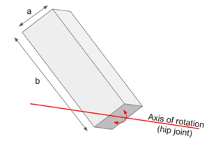
- For calculating moment of inertia of upperbody, it is assumed to be a parallelepiped (as shown in Figure 3.18).
- The lifting action from 70 to 10 degrees of trunk angle takes place for 1 second and sampling rate for calculation of desired position, velocity and torque is 60 Hz.
- The desired angular acceleration and external torque from the hip muscles are shown in fig. 3.18.

Created by Rahul Narasimhan Raghuraman based on [27]
Created by Rahul Narasimhan Raghuraman based on [29]
Equations
- Moment of Inertia of Upper body (refer Figure 3.19). Here I refers to mass moment of inertia, a refers to the depth and b refers to the length of the parallelepiped and M refers to upper body mass.
For the given model, a = 0.28 m, b = 0.66 m and M = 49.84 kg resulting in I = 7.56 kgm2
- Angular velocity. Here , , and t refers to angular velocity (current), initial angular velocity, angular acceleration, and time. All units are in SI.
- Angular displacement. Here refers to angular displacement.
- Impedance Control. Here, refers to the torque required from motors in the hip exoskeleton, K refers to stiffness constant, D refers to the damping coefficient, is the desired angular displacement, is the desired angular velocity, is the desired torque at the hip joint and is the external torque at the hip joint supplied by the human using hip muscles.
Pseudo Code
-
Initialize:
– j = handle of the leg joint that connects torso to legs
– timer = current simulation time
– theta = 0
– weight = weight of box + hands + forearms + upperarms + head + torso
– length = length of torso
– Inertia = mass moment of Inertia of upper body
– alpha_d1 = angular acceleration for the half of the lifting period
– alpha_d2 = angular acceleration for the second half of the lifting period
– torq_ext = external moment provided by the person using hip muscles
– K = stiffness constant
– D = damping coefficient
– vel_d = initial desired velocity
– pos_d = initial desired position
-
Actuation:
First half of lifting
while simulation time minus timer is greater than or equal to 0.017 and simulation time is less than or equal to 0.5:
– pos = current joint position
– vel = current joint velocity
– torq_d = desired torque value for completing the lifting action
– torq = impedance controller to set joint target force
– theta = angle covered
– pos_d = desired position
– torq_ext = external moment
– vel_d = desired velocity
– update timer
– print reference position
Second half of lifting
while simulation time minus timer is greater than or equal to 0.0017 and simulation time is less than or equal to 1:
– pos = current joint position
– vel = current joint velocity
– torq_d = desired torque value for completing the lifting action
– torq = impedance controller to set joint target force
– theta = angle covered
– pos_d = desired position
– torq_ext = external moment
– vel_d = desired velocity
– update timer
– print reference position
End simulation
if simulation time is greater than or equal to 1:
stop simulation
Link to github to download the coppeliasim model (ttt extension) with a non-threaded python child script attached – https://github.com/ClemsonSpring2023ME8930IntroRoboticsHRI/Ch3_ForceControl
Upon running this simulation, the lifting action should be complete with the assistance of a hip based exoskeleton using an impedance controller. Figure 3.20 illustrates this task.

Created by Rahul Narasimhan Raghuraman using [28]
Practice Problems
- What is the difference between passive and active interaction control?
Active Interaction Control:
This type of control involves actively applying forces/moments to manipulate the environment. This type of control may make use of sensors, feedback controls to generate forces/moments that is appropriate. It is commonly used in tasks that require precision control like assembly, manipulation and where the robot has to actively push, grasp or move objects in the environment.
Passive Interaction Control:
Passive interaction control, on the other hand, involves designing the robot or its end-effector to be compliant to external forces. Instead of active force application, mechanical design or the compliance of the robot allows it to naturally respond to external forces. Compliant materials such as springs, soft materials can be used for such use. By passive absorption or by dampening external forces safe and adaptive interaction with the environment is enabled. This type of control is common where human robot interaction is involved and sometimes it is used in combination with active based control.
- What type of force controller might be best suited for a task where both interaction force with the object and environment and the trajectory is also important?
Hybrid Motion/Force Control
- For the given block diagram provide the corresponding equation.
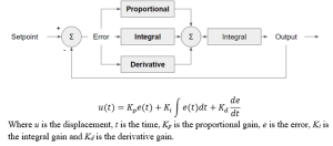
Created by Rahul Narasimhan Raghuraman based on information from [31]
Where u is the displacement, t is the time, Kp is the proportional gain, e is the error, Ki is the integral gain and Kd is the derivative gain.
References
- Ajoudani, Arash, Andrea Maria Zanchettin, Serena Ivaldi, Alin Albu-Schäffer, Kazuhiro Kosuge, and Oussama Khatib. 2018. “Progress and Prospects of the Human–Robot Collaboration.” Autonomous Robots 42 (5). https://doi.org/10.1007/s10514-017-9677-2.
- Alabdulkarim, Saad, and Maury A. Nussbaum. 2019. “Influences of Different Exoskeleton Designs and Tool Mass on Physical Demands and Performance in a Simulated Overhead Drilling Task.” Applied Ergonomics 74 (January): 55–66. https://doi.org/10.1016/J.APERGO.2018.08.004.
- Ali, Athar, Vigilio Fontanari, Werner Schmoelz, and Sunil K. Agrawal. 2021. “Systematic Review of Back-Support Exoskeletons and Soft Robotic Suits.” Frontiers in Bioengineering and Biotechnology 9 (November): 1027. https://doi.org/10.3389/FBIOE.2021.765257/BIBTEX.
- Al-Shuka, Hayder F.N., Steffen Leonhardt, Wen Hong Zhu, Rui Song, Chao Ding, and Yibin Li. 2018. “Active Impedance Control of Bioinspired Motion Robotic Manipulators: An Overview.” Applied Bionics and Biomechanics. Hindawi Limited. https://doi.org/10.1155/2018/8203054.
- “Back Injuries Prominent in Work-Related Musculoskeletal Disorder Cases in 2016 : The Economics Daily: U.S. Bureau of Labor Statistics.” n.d. Accessed February 15, 2023. https://www.bls.gov/opub/ted/2018/back-injuries-prominent-in-work-related-musculoskeletal-disorder-cases-in-2016.htm.
- Costa, Bruno R. Da, and Edgar Ramos Vieira. 2010. “Risk Factors for Work-Related Musculoskeletal Disorders: A Systematic Review of Recent Longitudinal Studies.” American Journal of Industrial Medicine 53 (3): 285–323. https://doi.org/10.1002/AJIM.20750.
- Crea, Simona, Philipp Beckerle, Michiel De Looze, Kevin De Pauw, Lorenzo Grazi, Tjaša Kermavnar, Jawad Masood, et al. 2021. “Occupational Exoskeletons: A Roadmap toward Large-Scale Adoption. Methodology and Challenges of Bringing Exoskeletons to Workplaces.” Wearable Technologies 2. https://doi.org/10.1017/wtc.2021.11.
- Duan, Jinjun, Yahui Gan, Ming Chen, and Xianzhong Dai. 2018. “Adaptive Variable Impedance Control for Dynamic Contact Force Tracking in Uncertain Environment.” Robotics and Autonomous Systems 102. https://doi.org/10.1016/j.robot.2018.01.009.
- Duchaine, Vincent, and Clément M. Gosselin. 2007. “General Model of Human-Robot Cooperation Using a Novel Velocity Based Variable Impedance Control.” In Proceedings – Second Joint EuroHaptics Conference and Symposium on Haptic Interfaces for Virtual Environment and Teleoperator Systems, World Haptics 2007. https://doi.org/10.1109/WHC.2007.59.
- “Force Control.” 2009. Advanced Textbooks in Control and Signal Processing, no. 9781846286414: 363–405. https://doi.org/10.1007/978-1-84628-642-1_9/COVER.
- Hogan, Neville. 1985. “Impedance Control: An Approach to Manipulation: Part I-Theory.” Journal of Dynamic Systems, Measurement and Control, Transactions of the ASME 107 (1). https://doi.org/10.1115/1.3140702.
- Ishmael, Marshall K., Andrew Gunnell, Kai Pruyn, Suzi Creveling, Grace Hunt, Sarah Hood, Dante Archangeli, K. Bo Foreman, and Tommaso Lenzi. 2022. “Powered Hip Exoskeleton Reduces Residual Hip Effort without Affecting Kinematics and Balance in Individuals with Above-Knee Amputations During Walking.” IEEE Transactions on Biomedical Engineering, October, 1–13. https://doi.org/10.1109/TBME.2022.3211842.
- Keemink, Arvid Q.L., Herman van der Kooij, and Arno H.A. Stienen. 2018. “Admittance Control for Physical Human–Robot Interaction.” International Journal of Robotics Research 37 (11). https://doi.org/10.1177/0278364918768950.
- Looze, Michiel P. de, Tim Bosch, Frank Krause, Konrad S. Stadler, and Leonard W. O’Sullivan. 2016. “Exoskeletons for Industrial Application and Their Potential Effects on Physical Work Load.” Ergonomics 59 (5): 671–81. https://doi.org/10.1080/00140139.2015.1081988.
- Madinei, Saman, Mohammad Mehdi Alemi, Sunwook Kim, Divya Srinivasan, and Maury A. Nussbaum. 2020a. “Biomechanical Evaluation of Passive Back-Support Exoskeletons in a Precision Manual Assembly Task: ‘Expected’ Effects on Trunk Muscle Activity, Perceived Exertion, and Task Performance.” Human Factors 62 (3): 441–57. https://doi.org/10.1177/0018720819890966.
- ———. 2020b. “Biomechanical Assessment of Two Back-Support Exoskeletons in Symmetric and Asymmetric Repetitive Lifting with Moderate Postural Demands.” Applied Ergonomics 88 (October). https://doi.org/10.1016/j.apergo.2020.103156.
- Madinei, Saman, Sunwook Kim, Divya Srinivasan, and Maury A. Nussbaum. 2021. “Effects of Back-Support Exoskeleton Use on Trunk Neuromuscular Control during Repetitive Lifting: A Dynamical Systems Analysis.” Journal of Biomechanics 123 (June). https://doi.org/10.1016/j.jbiomech.2021.110501.
- O’Hara, G. J. 1967. “Mechanical Impedance and Mobility Concepts.” The Journal of the Acoustical Society of America 41 (5). https://doi.org/10.1121/1.1910456.
- Ortenzi, V., R. Stolkin, J. Kuo, and M. Mistry. 2017. “Hybrid Motion/Force Control: A Review.” Advanced Robotics 31 (19–20). https://doi.org/10.1080/01691864.2017.1364168.
- “Principles of Force Control · Introduction to Open-Source Robotics.” n.d. Accessed April 25, 2023. http://www.osrobotics.org/osr/control/principles.html.
- Raibert, M. H., and J. J. Craig. 1981. “Hybrid Position/Force Control of Manipulators.” Journal of Dynamic Systems, Measurement, and Control 103 (2): 126–33. https://doi.org/10.1115/1.3139652.
- Theurel, Jean, and Kevin Desbrosses. 2019. “Occupational Exoskeletons: Overview of Their Benefits and Limitations in Preventing Work-Related Musculoskeletal Disorders.” IISE Transactions on Occupational Ergonomics and Human Factors 7 (3–4): 264–80. https://doi.org/10.1080/24725838.2019.1638331.
- Wei, Meng, Quan Liu, Zude Zhou, and Qingsong Ai. 2014. “Active Interaction Control Applied to a Lower Limb Rehabilitation Robot by Using EMG Recognition and Impedance Model.” Industrial Robot 41 (5). https://doi.org/10.1108/IR-04-2014-0327.
- “Work Injury Costs – Injury Facts.” n.d. Accessed April 25, 2023. https://injuryfacts.nsc.org/work/costs/work-injury-costs/.
- Yamakawa, H., H. Hosaka, H. Osumi, and K. Itao. 2001. “Development of a System for Measuring Structural Damping Coefficients.” Human Friendly Mechatronics, 259–64. https://doi.org/10.1016/B978-044450649-8/50044-9.
- Zeng, Ganwen, and Ahmad Hemami. 1997. “An Overview of Robot Force Control.” Robotica 15 (5): 473–82. https://doi.org/10.1017/S026357479700057X.
- Winter, David. 1990. “Biomechanics and Motor Control of Human Movement.” Choice Reviews Online 28 (04): 28–2135. https://doi.org/10.5860/choice.28-2135.
- “CoppeliaSim – Coppelia Robotics.” https://www.coppeliarobotics.com/coppeliaSim.
- Zagrevskiy, V. I., and O. I. Zagrevskiy. “Spatial model of biomechanical system: Geometric transformations.” Theory and Practice of Physical Culture 8 (2016): 27-27.
- Fryar, Cheryl D., Qiuping Gu, Cynthia L. Ogden, and Katherine M. Flegal. “Anthropometric reference data for children and adults; United States, 2011-2014.” (2016).
- Mehta, Nikunj, Dharmendra Chauhan, Sagar Patel, and S. Mistry. “Design of HMI based on PID Control of Temperature.” International Journal of Engineering Research and 6 (2017): 05.
