
2 Inverse Kinematics and Motion Control of Robots in Aerospace Manufacturing
Emma Brandberg
Chapter Outline
2.1 Introduction
2.2 Kinematics Model of Robots in Aerospace Manufacturing
2.3 Differential Kinematics
2.3.1 Analytical Jacobian
2.3.2 Geometric Jacobian
2.4 Inverse Differential Kinematics
2.5 Joint Space Motion Control with Velocity Inputs of Robots in Aerospace Manufacturing
2.6 Summary
2.7 Practice Problems in Aerospace
2.8 References
2.1 Introduction
Industrial robots are growing in popularity across the world, and in return, growing more technologically advanced every day. The automotive industry is paving the way for other industries, such as aerospace, as it uses both collaborative and programmed robots (see Figure 2.1). Collaborative robots allow employees to work alongside robots in the same workspace, and they learn tasks via human demonstration and mimicking. On the contrary, programmed robots are typically in a locked-out environment when they perform tasks and require programming to perform tasks [2]. Aerospace manufacturers can seek guidance from automotive manufacturers regarding their utilization of robots to perform jobs on varying models of automobiles. Similarly to how Toyota has varying models such as the Camry, Corolla, etc., Boeing has the 737, 777, and 787.

“KUKA Industrial Robots IR” by Mixabest is licensed under CC BY-SA 3.0.
The aerospace industry is looking eagerly to the advancements of robots, as they can be applied to many facets of the manufacturing process. However, there are reasons why aerospace is relatively new to robot inclusion compared to the automotive industry. For starters, aerospace products, such as commercial airplanes, fighter jets, and autonomous vessels, require high positional accuracy for their complex builds. Along with their strict tolerances, these aircrafts are generally far larger in size compared to automobiles. Despite these obstacles, the aerospace industry needs manufacturing enhancements to create a leaner process, and robots have potential to deliver [1].
Robots can be utilized in the aerospace community to drill and fasten fasteners into the fuselage, paint the aircraft, weld, inspect suspected damaged areas, and even retrieve and dispense pertinent tools to perform jobs (see Figure 2.2). Drilling and fastening are areas of great focus due to the strain the current methods pose to the human body. There are hundreds of thousands (sometimes even millions) of fasteners on commercial jets, and they are successfully installed through awkward positions, heavy tools, high torque values to pass quality requirements, etc. Introducing robots to drill and fasten would mean less injuries, higher quality and more reproducible work, and faster production. The downsides of introducing a robot system are the risk of unplanned downtime if the robot malfunctions, the need for a numerical programmer to code and maintain the robot, the cost, and the lead time. A common misconception in the manufacturing environment is that introducing robots will reduce job security. This assumption can be overturned with the idea of robots being a rate enabler. This means with a higher production rate; humans will be needed in other areas of production that cannot be automated. Also, letting robots take over ergonomically daunting, time consuming, mindless tasks gives employees more time to utilize their skills in other realms.
For an aerospace manufacturer to choose the ideal robot for their application, they must first understand the constraints and requirements of their workspace. If a robot is working to build, repair, or inspect an aircraft, it is critical to never put the aircraft in danger of (more) damage. This is why it is important to robustly define the controls of one’s robot. The following chapter will delve into velocity-based motion controls of robots in aerospace and the kinematic, foundational knowledge required to understand said motion controls.

“At Boeing’s Everett factory near Seattle” by Jetstar Airways is licensed under CC BY-SA 2.0.
2.2 Kinematics Model of Robots in Aerospace Manufacturing
Velocity-based control is of particular interest to the aerospace industry for applications that involve minimal to no force or perform tasks at a predictable, steady force. With the elimination of force needing to be controlled, we can focus on the joint velocities of the manipulator to successfully perform tasks. A paint booth with an end-effector that sprays and therefore does not apply force to the surface it is painting, is an application for velocity-based controls. To understand velocity-based control of manipulators, we must first understand the kinematic model of such a robot.
In robot kinematics, a model can be created through the mapping between the task space and joint space. To create a kinematic model of a robot, one must know the type of joints existing within the robot, the lengths of the links between the joints, and their position and orientation relative to each other. The two types of joints are revolute and prismatic. Prismatic (P) joints allow for displacement along a common axis and have one degree of freedom (DoF). Revolute (R) joints allow for rotation about a common axis and have one DoF.
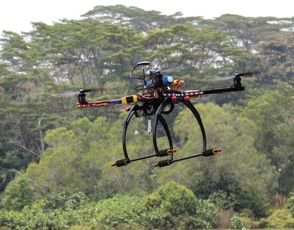
The style of robot in Fig. 2.1 would be commonly found in the aerospace industry. A common manufacturer of these robots is KUKA, whose robots can be seen to aid in installation of fasteners through programming, as well as work alongside humans while parts are loaded onto an assembly line. Now that the types of joints in a robot are understood, let us look at a articulated (RRR) robotic arm kinematic model in the figure below.

Created by Emma Brandberg
With all the frames labeled along with their respective orientations and positions to each other, Denavit–Hartenberg parameters can be found via the DH table (twist angles, link lengths, joint displacements, and link offsets) [3]. The position and orientation of the ith coordinate frame with respect to (i-1) can be found using the homogeneous transformation matrix as depicted below in Equation (2.1), where R is the special orthogonal group and d is a set of real values (3 dimensions).

The forward kinematics (FK) of the RRR robot can be computed once the DH table and homogeneous transformation matrix are found. Please refer to Chapter 2 in [6] for details on finding the FK. As for the inverse kinematics (IK), either the algebraic, geometric, or numerical approach can be utilized to find the joint variables when the end-effector position and orientation are known. Please refer to Chapter 3 in [7] for details on finding the IK.
2.3 Differential Kinematics
Differential kinematics (DK) allow for instantaneous motion analysis. DK is mapping of the tangent space of the configuration space into the tangent space of the workspace of the end-effector. By taking the derivative of the forward map in forward kinematics (FK), the analytical Jacobian can be produced.
2.3.1 Analytical Jacobian
The analytical Jacobian, ![]() , is the gradient of forward kinematics and is defined by Equation (2.2) below.
, is the gradient of forward kinematics and is defined by Equation (2.2) below.

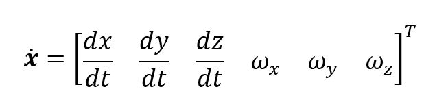
Take the time derivative on both sides of the equation and the result is Equation (2.3):

![]() and
and ![]() are represented below.
are represented below.  ,
,  , and
, and  are roll, pitch, and yaw rates with respect to the base frame.

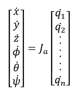
![]() can then be related to the analytical Jacobian with respect to all the joint positions with Equation (2.4).
can then be related to the analytical Jacobian with respect to all the joint positions with Equation (2.4).
Example analytical Jacobian in DK:
Given the below Revolute Prismatic (RP) robotic arm, find the DK using the analytical Jacobian:

Created by Emma Brandberg
The DH table can be used to find the DH parameters and then the FK. See the FK below:

Next, take the time derivative on both sides of the equations, and arrive at the DK:

2.3.2 Geometric Jacobian
The geometric Jacobian, ![]() , is no longer talking about the roll, pitch, and yaw rate with respect to the base frame. Rather, we are talking about the angular velocity,
, is no longer talking about the roll, pitch, and yaw rate with respect to the base frame. Rather, we are talking about the angular velocity, ![]() , with respect to the body fixed framework of the end-effector. The geometric Jacobian is the more straight forward way to control the motion of the end-effector. The geometric Jacobian can be related to the angular velocities via the joint velocities, as stated in Equation (2.5) below.
, with respect to the body fixed framework of the end-effector. The geometric Jacobian is the more straight forward way to control the motion of the end-effector. The geometric Jacobian can be related to the angular velocities via the joint velocities, as stated in Equation (2.5) below.

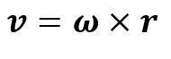
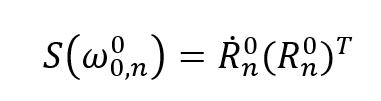
First, one must recall angular velocity, ![]() . Angular velocity is a vector measure of rotation rate about an axis. Angular velocity can be related to linear velocity by Equation (2.6) below, where
. Angular velocity is a vector measure of rotation rate about an axis. Angular velocity can be related to linear velocity by Equation (2.6) below, where ![]() is the distance of a point with respect to the origin.
is the distance of a point with respect to the origin.
Next, one must understand the angular velocity Jacobian, ![]() . There are 2 different cases of finding
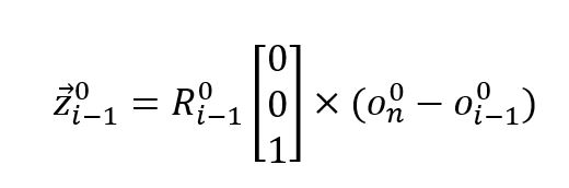
. There are 2 different cases of finding ![]() , depending on the type of joint, i. If i is revolute, then the rate of rotation is
, depending on the type of joint, i. If i is revolute, then the rate of rotation is ![]() , and the axis of rotation is
, and the axis of rotation is ![]() with respect to frame {i-1} expressed in {0}. With this knowledge, the equation below can be stated.
with respect to frame {i-1} expressed in {0}. With this knowledge, the equation below can be stated.

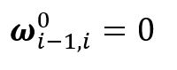
On the contrary, if i is prismatic, then frame {i} translates with respect to frame {i-1} expressed in {0}, and there is no rotation. This is represented by Equation (2.8) below.
For angular velocity, one only needs to care about rotational joints. The end-effector velocity can be found by Equation (2.9) below.

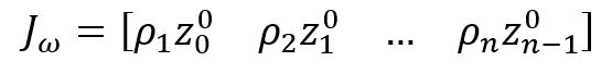
The angular velocity Jacobian, ![]() , can be represented as Equation (2.10) below.
, can be represented as Equation (2.10) below.
Next, the linear velocity Jacobian, ![]() , must be derived. It is known that o is the displacement vector. Below is the relationship between
, must be derived. It is known that o is the displacement vector. Below is the relationship between ![]() and o.
and o.

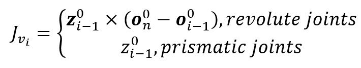
If i is prismatic, the end-effector translates along ![]() with velocity
with velocity ![]() , represented by the equations below.
, represented by the equations below.


If i is revolute, linear velocity is given by Eqn. 2.6 where the below relationships exist, where r is the position vector from joint i to the end-effector.


The linear velocity Jacobian, ![]() , can be represented by the below.
, can be represented by the below.

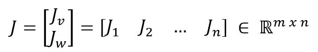
Therefore, the geometric Jacobian can be found by the below relationships. The number of rows in a matrix is m and the number of columns is n. Usually, m = 6 and n = the number of joints.

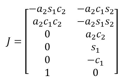
Geometric Jacobian example:

Created by Emma Brandberg
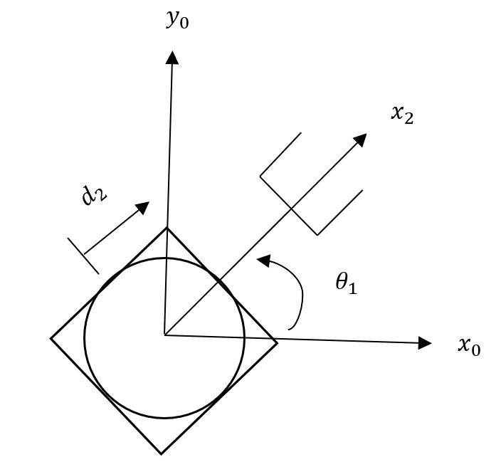
Created by Emma Brandberg
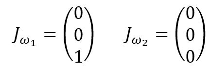
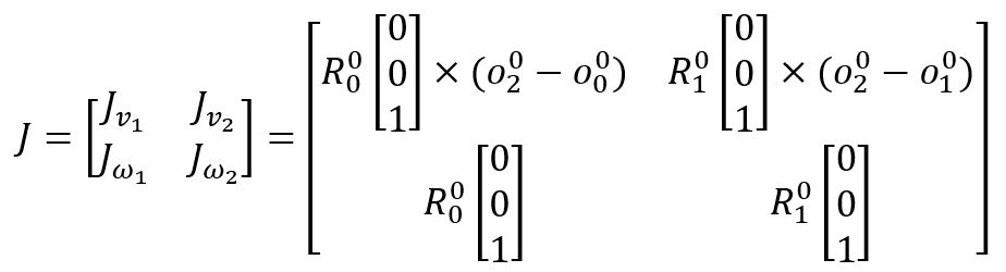
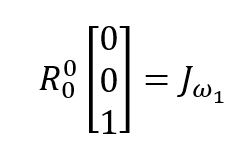
First, calculate angular velocity:
Now, calculate linear velocity:
When joint 1 is moving,

When joint 2 is moving,
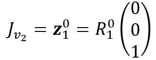
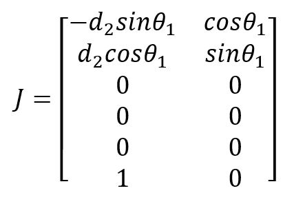
The geometric Jacobian can then be found:
Now that the analytical and geometric Jacobians are derived and understood, let’s identify the key similarities and differences between them:
- Both Jacobians are matrices that relate joint velocities,
 , with workspace velocities.
 - Both geometric and analytical Jacobians will give the same result for linear velocities, but the result is different for angular velocities.
- If the analytical Jacobian is used, the time derivative of roll, pitch, and yaw angles is derived, i.e., roll, pitch, and yaw rates.

- If the geometric Jacobian,
 , is used, the angular velocities around the x, y, and z (rotation between 2 frames) is obtained.
- Angular velocity does not have an integral-like associated term, such as angular position. Angular velocities can be represented as a function of roll, pitch, and yaw rates.
2.4 Inverse Differential Kinematics
Inverse differential kinematics (IDK) raises the question of: If you want to control the velocity of your end-effector, what should be your joint velocity of the manipulator? Joint velocity is the most popular control input to give a robot manipulator. Let us learn how to find the IDK below.
We know that (for either analytical or geometric Jacobian) if ![]() , then
, then ![]() . If
. If ![]() is square and hence invertible,
is square and hence invertible, ![]() . If
. If ![]() , rank
, rank ![]() ,
,
- If rank
 is full row rank, rank
  (too few equations
  invertible)
 - If rank
 is full column rank,
  rank (too many equations
  invertible)
Inverse Differential Kinematics Example:

Created by Emma Brandberg
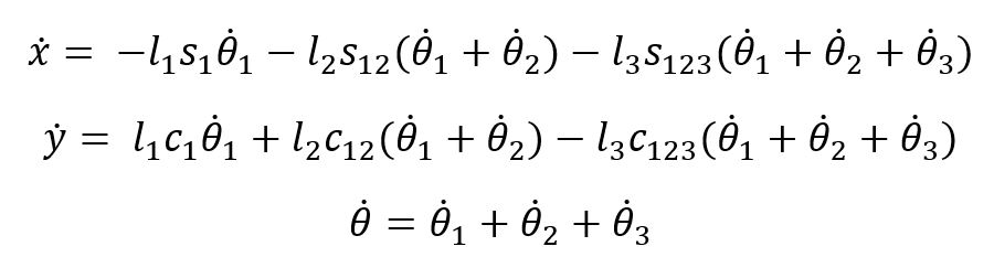
FK are given as:

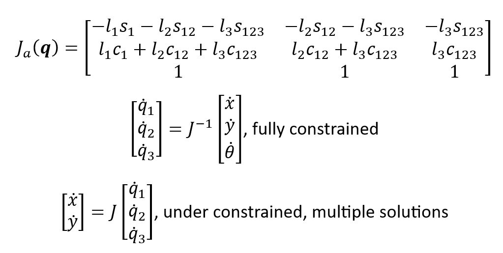
Let’s use the analytical Jacobian, ![]() , to find the IDK.
, to find the IDK.
![]() is fully constrained with the end-effector velocities.
is fully constrained with the end-effector velocities.
Now, let us discuss the pseudoinverse of ![]() .
.
The right pseudoinverse, ![]() , is to the right of the Jacobian matrix. The right pseudoinverse has an infinite number of solutions (too few equations, under constrained).
, is to the right of the Jacobian matrix. The right pseudoinverse has an infinite number of solutions (too few equations, under constrained).

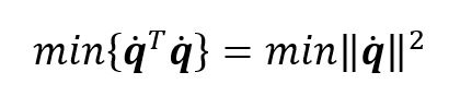
Given the workspace velocities, ![]() , the least effort joint velocities can be found with the following equation.
, the least effort joint velocities can be found with the following equation.
If the right pseudoinverse cannot be found, you can write ![]()
The right pseudoinverse satisfies the Moore-Penrose conditions: ![]()

The left pseudoinverse, ![]() , is to the left of the Jacobian matrix. The left pseudoinverse may have no solution (too many equations, over constrained).
, is to the left of the Jacobian matrix. The left pseudoinverse may have no solution (too many equations, over constrained).
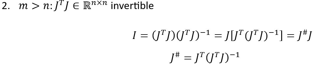
If the left pseudoinverse cannot be found, you can write ![]() .
.
The left pseudoinverse satisfies the Moore-Penrose conditions: ![]()

Now we must ask the following question; If we have a Jacobian matrix of dimensions m x n (not full rank), how will we define the singular configuration?
Singular configuration:

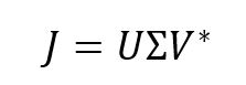
The singular value decomposition (SVD) of a matrix, ![]() , is a very powerful method to find the pseudoinverse. SVD can be applied to any general matrix, regardless of the size. Step 1 in the SVD method is to rewrite the matrix,
, is a very powerful method to find the pseudoinverse. SVD can be applied to any general matrix, regardless of the size. Step 1 in the SVD method is to rewrite the matrix, ![]() , in terms of the multiplication of its left singular vector, right singular vector, and diagonal matrix,
, in terms of the multiplication of its left singular vector, right singular vector, and diagonal matrix, ![]() . See the equation below.
. See the equation below.
*Represent conjugate transpose,

Note: bolded variables are vectors
The Moore-Penrose pseudoinverse is given by the following equations when m < n. This gives us the joint velocity in terms of end-effector velocity.
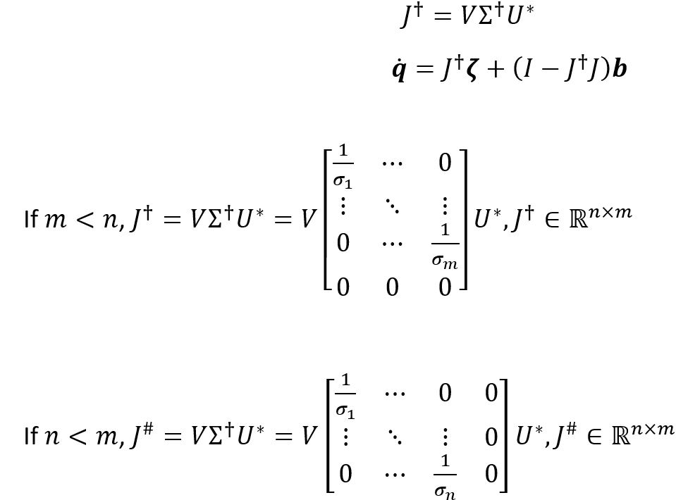
Solving for the pseudoinverse of the Jacobian allows us to find IDK for velocity-based control. In the next section, we will explore joint space motion control with velocity inputs in aerospace manufacturing.
2.5 Joint Space Motion Control with Velocity Input of Robots in Aerospace Manufacturing
Motion control is when you move a robot with no requirements other than following a certain trajectory. The trajectory of the motion control can be expressed in joint space or task space. Joint space motion control is when the controller is fed a steady stream of desired joint positions ![]() , and the goal is to command joint velocities or torque/force that cause robot to track this trajectory. Task space motion control is when the controller is fed a steady stream of end-effector configurations
, and the goal is to command joint velocities or torque/force that cause robot to track this trajectory. Task space motion control is when the controller is fed a steady stream of end-effector configurations ![]() , and the goal is to command joint velocities or torque/force that cause the robot to track this trajectory. It is more common to have task space motion control because the end-effector location is usually more critical than where each of the joints are. However, in this section we are going to focus on joint space motion control with velocity input.
, and the goal is to command joint velocities or torque/force that cause the robot to track this trajectory. It is more common to have task space motion control because the end-effector location is usually more critical than where each of the joints are. However, in this section we are going to focus on joint space motion control with velocity input.
In joint space motion control with velocity inputs, we assume that the robot is velocity controlled, meaning the robot can be programmed with velocity inputs. Actuators are stepper motors, and they can be utilized to determine the robot velocity based on the frequency of the pulse train sent to the stepper. Joint space motion control with velocity inputs is a good choice of motion control when the application is low or predictable in force-torque requirements. This is due to not being able to control the force in the joint space motion control with velocity inputs method.
The simplest case of joint space motion control with velocity inputs is with one joint (feedforward control). Consider a desired joint trajectory ![]() , the simplest type of control would be to choose the commanded velocity
, the simplest type of control would be to choose the commanded velocity ![]() as the below relationship.
as the below relationship.
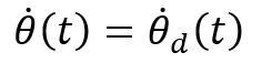
![]() comes from the desired trajectory. This is called a feedforward or open-loop controller since no feedback (sensor data) is needed to implement it.
comes from the desired trajectory. This is called a feedforward or open-loop controller since no feedback (sensor data) is needed to implement it.
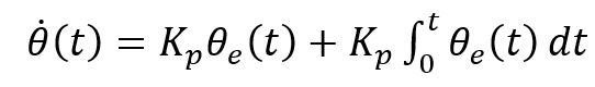
An alternative strategy is to measure the actual position of each joint continually and implement a feedback controller, e.g., a proportional controller. This is called the feedback control (single joint) method and is represented by the equation below.

The feedback controller method requires a sensor mounted on top of the robot to measure ![]() and compare it to
and compare it to ![]() .
.
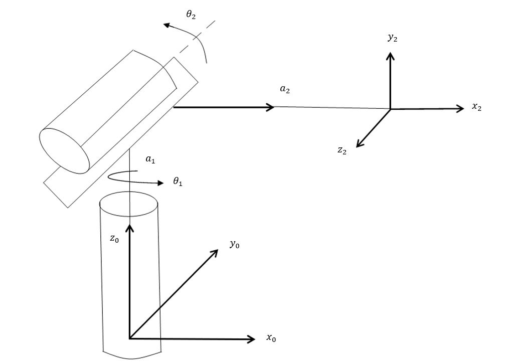
A more complex controller for a single joint is a proportional-integral (PI) controller. A PI controller allows you to eliminate errors while you try to achieve the designed control. A PI controller can be represented by the below equation.
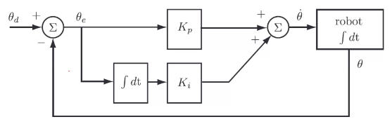
Created by Emma Brandberg
One downside of feedback control is that an error is required before the joint begins to move. It would be ideal to use the knowledge of the desired trajectory, ![]() , to initiate motion before any error occurs.
, to initiate motion before any error occurs.
The best method for joint space motion control with velocity inputs is a combination of feedforward and feedback control. This is ideal since the feedforward control commands motion without an error and feedback control mitigates accumulation of error. This combination for a single joint can be represented as follows:

Created by Emma Brandberg
Motion control of a multi-joint robot can utilize Equation (2.25) as well and be generalized to robots with n joints with both ![]() and
and ![]() as -vectors.
as -vectors.
Joint space motion control with velocity inputs can be observed in the aerospace industry in areas such as paint and pick and place zones. When painting the fuselage of an aircraft via robots, the force of the end-effector is not important because it does not actually contact the barrel. This makes velocity inputs an ideal motion control candidate for automated painting. The end-effector typically consists of a spray mechanism that sprays paint onto the barrel at a constant rate. While painting, the main priority is the path of the robot, which can be controlled via velocity inputs. If multiple robots are painting at a time, it is crucial for the robots to be equipped with collision avoidance. Collision avoidance usually entails a simulation that maps the planned trajectory prior to confirming the run. It also prevents robots from entering a programmed radius of each other via sensors.
Another application of joint space motion control with velocity inputs in the aerospace industry is the picking and placing of inventory. This application can be seen across many industries, not sure aerospace, but it is on the horizon as aerospace companies attempt to lean out their manufacturing processes with less reliance on humans for mundane tasks. Examples of picking and placing include loading items onto a conveyor belt at the start of an assembly line and picking fasteners from reservoirs and placing them in point of use areas for humans to use. Picking and placing applications do not require force control, as they are not required to apply a set amount of force to perform a job to specification, such as drilling an aircraft fuselage. Velocity control is a good candidate for collaborative robots as they typically will not put humans in danger of heavy force.
Joint space motion control with velocity inputs can be explored as a control type for autonomous flight. Many companies are on the brink of introducing autonomous flight vehicles to the world. These vehicles have varying applications, from refueling other jets while unmanned, to carrying crew and being remotely controlled from outside the vessel. Drones (Fig. 2.10) can be seen using joint space motion control with velocity inputs as they can be programmed to follow a path based on velocity inputs.
“Drone 2” by Michael Khor is licensed under CC BY 2.0.
2.6 Summary
The aerospace industry is eager to automate their processes that require little thought yet are ergonomically daunting to their employees. Joint space motion control with velocity inputs is a realm of robotics that can be explored while robots are continually being introduced to industry. Prior to understanding joint space motion control with velocity inputs, an understanding of the analytical and geometric Jacobian, differential kinematics, inverse differential kinematics, and pseudoinverse differential kinematics is necessary. Through application of joint space motion control with velocity inputs, the aerospace industry can reach new heights in advancing their technological capabilities while achieving tasks that require little to no force or consistent, predictable force.
2.7 Practice Problems
Exercises
- Given the RR robot manipulator, calculate the geometric Jacobian.
Created by Emma Brandberg
Solution:
First, recall the linear and rotational geometric Jacobian formulas below.
Linear:
Rotational:

Now, we can rewrite the Jacobian with the above elements included. We know that n = 2 since there are 2 joints.
We know that
Use the DH method to find ![]() and then find the homogeneous transformation matrix.
and then find the homogeneous transformation matrix.
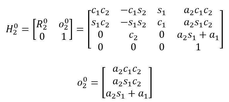
Next, we must find ![]()

Next, let’s find ![]()

Next, let’s find ![]()

Lastly, let’s combine them all to find the geometric Jacobian, ![]()
2. Explain the differences between task space motion control and joint space motion control.
Solution: Joint space motion control is when the controller is fed a steady stream of desired joint positions ![]() , and the goal is to command joint velocities or torque/force that cause robot to track this trajectory. Task space motion control is when the controller is fed a steady stream of end-effector configurations
, and the goal is to command joint velocities or torque/force that cause robot to track this trajectory. Task space motion control is when the controller is fed a steady stream of end-effector configurations ![]() , and the goal is to command joint velocities or torque/force that cause the robot to track this trajectory. The difference between them is what they are controlling, joint positions or end-effector configurations.
, and the goal is to command joint velocities or torque/force that cause the robot to track this trajectory. The difference between them is what they are controlling, joint positions or end-effector configurations.
3. Suppose that ![]() is a solution to
is a solution to ![]() for m < n. Show that
for m < n. Show that ![]() is also a solution for any
is also a solution for any ![]() .
.
Solution:

2.8 References
[1] Bogue, Robert. “The growing use of robots by the aerospace industry.” Industrial Robot: An International Journal (2018).
[2] Kragic, Danica, Joakim Gustafson, Hakan Karaoguz, Patric Jensfelt, and Robert Krug. “Interactive, Collaborative Robots: Challenges and Opportunities.” In IJCAI, pp. 18-25. 2018.
[3] Kostic, Dragan, Bram De Jager, Maarten Steinbuch, and Ron Hensen. “Modeling and identification for high-performance robot control: An RRR-robotic arm case study.” IEEE Transactions on Control Systems Technology 12, no. 6 (2004): 904-919.
[4] “File:Robot articulat.svg” by EBatlleP is licensed under CC BY-SA 3.0.
[5] “KUKA Industrial Robots IR” by Mixabest is licensed under CC BY-SA 3.0.
[6] Stevens, Ashley. “Forward Kinematics.” Modeling Motion Planning and Control of Manipulators and Mobile Robots, https://opentextbooks.clemson.edu/wangrobotics/chapter/forward-kinematics/.
[7] Lunia, Akshit. “Inverse Kinematics.” Modeling Motion Planning and Control of Manipulators and Mobile Robots, https://opentextbooks.clemson.edu/wangrobotics/chapter/inverse-kinematics/.
[8] “Drone 2” by Michael Khor is licensed under CC BY 2.0.
[9] “At Boeing’s Everett factory near Seattle” by Jetstar Airways is licensed under CC BY-SA 2.0.
