
4 Robot Path Planning and Application in Manufacturing Logistics
Ryan Mbagna-Nanko
Robot Path Planning and Application in Manufacturing Logistics
4.1 Introduction: Path planning and Controls definition.
- 4.1.1 Motivation
4.2 Methodology
- 4.2.0.1 Terminology
- 4.2.1 Grid-based methods
- 4.2.1.1 Dijkstra,
- 4.2.1.2 Uniform Cost Search (UCS),
- 4.2.1.3 A-Star (A*),
- 4.2.2 Sampling-based methods
- 4.2.2.1 Probabilistic RoadMap Planner (PRM),
- 4.2.2.2 Rapidly-exploring Random Tree (RRT),
- 4.2.2.3 Rapidly-exploring Random Tree – Star (RRT*)
4.3 Mobile Robot Design Setup
- 4.3.1 Simulation setup
4.4 Summary
4.5 Practice
4.6 Reference
4.1 Introduction: Path planning
Considering a manufacturing warehouse scenario, we study a collaboration between human operators and mobile robots. In a case where humans rely on mobile robots to transport and deliver goods in a timely manner, it is imperative that these robots be autonomous and self-sufficient. Meanwhile, the human operator is the extension of the mobile robots for enhanced manipulation, and added flexibility. At this scale, this would require managing multiple mobile robots based on their objective, while avoiding the collision with the environment, including the human handler and other mobile robots. Assuming that the nature of a warehouse is a controlled space, and the layout is not likely to change. This presents an opportunity to explore offline path planning given that any given robot would have complete knowledge of its whereabouts and its environment.
In the context of robotics, there are multiple ways we can define a path of a mobile robot, and optimize its route to the end point. This chapter will explore offline path planning methods and demonstrate its use case with multiple mobile robots in a manufacturing setting. As we move from one point to another, the goal is to engage with you as we breakdown each path planning methodologies. Feel free to interact with the corresponding modules provided, which include a sample python code and an interaction with the mobile robot via Coppelia-Sim. You can use these resources to practice your coding skills and deepen your understanding of the algorithms covered in any section. So don’t hesitate to dive in and experiment with the concepts to enhance your knowledge of path planning algorithms. In addition, a few exercises are provided to test your understanding. With that in mind, let’s get started.
4.1.1 Motivation:
In recent years, reports showcase growing trends in the e-commerce industry that use warehouse robots to cope with the high number of sales and delivery targets [8]. The consensus is to support human labor and maintain efficiency targets by automating navigation and translation of goods. According to a survey conducted by BIBA in 2007, the area of robotics-logistics fulfills a great need for modernization.
Warehouse robots in the logistics industry have grown more favorably. This includes the complete planning, controlling, realization and testing of all institutions’ internal and overlapping flow of goods and personnel [8]. For instance, in May 2020, United Parcel Services unveiled new warehouse network technology called Warehouse Execution System (WES). It uses autonomous mobile robots (AMRs) to enable faster order intake and fulfillment.
In the general sense, robotics logistics falls in the scope of motion planning. In this case, the objective is for the robot to navigate itself, either in 2D or 3D space, while avoiding obstacles in the environment, to meet its end goal. Path planning is the sub-group of motion planning. Path planning focuses on a geometric-based solution to finding a collision-free path without concerning dynamics and motion duration. Path planning plays a critical part in manufacturing logistics primarily for: optimizing delivery time by reducing distance traveled, reduction of collision by avoiding obstacles, and aiding in system-wide coordination of multiple robots.
4.2 Methodology
This section presents different methodologies focusing on path planning. We will cover two popular classifications: the grid-based algorithms (see Section 4.2.1 , which lists the most important grid-based algorithms, their advantages and drawbacks); the sampling-based techniques (see Section 4.2.2, which explains the advantages of sampling based methods for high-dimensional space in the path planner design). Lastly, we will introduce multi-robot path planning (see Section 4.3, which will showcase how multi-robot collaboration comes into play).
4.2.0.1 Terminology
Given the technical nature of this chapter, let us first break down common gerunds used throughout.
The working environment can be defined as the configuration space, Cspace. This is where the robot operates. The presence of obstacles creates two separate spaces in the Cspace, namely free Cspace (Cfree) and obstacle space (Cobs), where the combination of these two is the entire Cspace (C = Cfree ∪ Cspace). The existence of obstacles may cause Cfree to be divided into multiple linked parts. In such cases, it may not be possible to find a viable path between configurations in different linked components.
When dealing with Cspace, the majority of path planning techniques use a graph format, which comprises “Nodes” and “Edges”. In the context of data structures, a “Graph” is a depiction of the links between two or more items known as “Nodes” or vertices, which are usually real-time objects, persons or entities. Meanwhile, “Edges” are the straight-line links between nodes [4].
A path planning algorithm can be thought of as a map, where the nodes represent key points and the edges represent the paths connecting them. This mapping creates a clear and structured pathway for the robot to navigate from the starting point to the end point. By utilizing this map, the robot can plan its path and reach its destination in a more efficient manner. Regarding search algorithms, we can classify each approach in two ways. The first is based on its ability to produce the lowest-cost path, which we refer to as “optimal.” The second is whether the algorithm explores the entire Cspace, which we refer to as “complete.”
To further illustrate this concept, we will be using a simple tool called Graph Online. This tool will help us to depict a simple path planning problem for each algorithm discussed. By using Graph Online, you can easily create your own graphs and test yourself by attempting to solve each problem the same way as the algorithms. In addition, a sample code for each discussed model is compiled via GitHub (https://github.com/ClemsonSpring2023ME8930IntroRoboticsHRI/Ch4_Path_Planning).
4.2.1 Grid-based methods
These methods discretize the workspace (Cfree) into a grid and form a graph for these grids, then search an optimal path from the start node to the goal node. These methods are relatively easy to implement and can return optimal solutions but, for a fixed resolution, the memory required to store the grid, and the time to search it, grow exponentially with the number of dimensions of the space. This limits the approach to low-dimensional problems [2].
4.2.1.1 Dijkstra
This algorithm is used to find the shortest distance, or minimum cost path. By exploring all possible weighted nodes, the goal is to follow the path that weighs the least [4]. Unlike most other search algorithms discussed, Dijkstra does not have a specific target node, but is applied to every other node in the Cspace. The steps are as follows:
- All costs are set to infinity at the beginning and the starting node is set to zero. This is done to make sure that every other cost we may compare it to would be smaller than the starting one because it has no path to itself.
- We create a list of visited nodes, to keep track of all nodes that have been assigned their shortest paths.
- When we pick a node with the shortest current cost, it is added to the list of visited nodes.
- The costs are updated for all adjacent nodes that are not visited yet. We do this by comparing its old cost with the sum of the parent’s node and the cost of the edge between the parent node and the adjacent node

Algorithm 4.1. Dijkstra-Algorithm, Created by Ryan Mbagna-Nanko based on information from Modern Robotics [2].
Below is an example: A mobile robot wants to calculate the shortest distance between the start, G, and the goal, G, while calculating a subpath which is also the shortest path between its source and destination. With the graph provided below, use the Dijkstra method to determine the shortest distance traveled by the mobile robot to its destination.
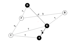
Figure. 4.1. Dijkstra-algorithm illustration. Solved example made using GraphOnline, Created by Ryan Mbagna-Nanko based on information from Modern Robotics [2] [4]
Solution
As a result, node E is the shortest path to G. The main advantage of the Dijkstra algorithm is that it is straightforward and little in complexity. We can compare multiple pathways to determine the shortest line to the desired end point. On the other hand, it is time consuming. This is because the Dijkstra algorithm must keep track of the changing index of the nodes, while taking into account their weights. This method is not always accurate in determining the shortest path, since it also cannot handle negative edges either. In a practical sense, this method can help the mobile robot in a manufacturing plant determine the shortest distance to its handler. However, its processing time may take longer than expected considering the multiple routes it must map first.
4.2.1.2 Uniform Cost Search (UCS)
Uniform Cost Search is a variant to Dijkstra. The Dijkstra algorithm prioritizes distance and chooses shortest paths from the starting node to every other node in a graph. While the UCS algorithm assumes the cost towards the goal is uniform, the overall cost of a set path is defined as the sum of all the paths. This means the algorithm aims to find the path with the lowest cost from the starting point to the goal point by exploring adjacent states. It chooses the least costly state from all the non-visited and adjacent states of the visited states, and continues searching for other possible paths even if the goal state is reached. A priority queue is maintained to determine the least costly next state from all the adjacent states of the visited states. This becomes useful when a graph becomes too large for Dijkstra to fully map out. As a result, we get an optimal solution since the least path at each iteration is followed [6]. The steps are as follows.
- Let us define a list, pathCost, to store the total cost of a path. Similarly, we define a list, pathOpen, to store the nodes configuration with the least total cost from start to goal point.
- For every iteration, the path configuration expands to include the current node and pathCost is updated accordingly.
- If this node is the goal node, return the path to the goal node.
- else, expand the path by generating all of its neighbors and calculate the cost to reach each neighbor.
- For each neighbor, if the cost to reach it is less than its current cost, update the neighbor’s cost and put it on the priority queue.
- Repeat steps 3-6 until the goal node is reached.

Algorithm 8.2. UCS-Algorithm, Created by Ryan Mbagna-Nanko based on information from Medium [6].
The terminology used in the pseudocode Algorithm 8.2:
Here, pathOpen and pathClosed are priority queues. Priority queues are abstract data structures where each data/value in the queue has a certain priority. The queue is modified at every iteration using functions In priority queues, .pop(), is used to remove the last element of the list, and insert(location,value) is used to insert the value in the specified location. Here the cost is initially considered as zero. Every time we reach the child node, the cost is added based on the edge value.
The graph given below represents a simple scenario in which a mobile robot needs to find the shortest path between its starting point, S, and its destination, G. The graph consists of several nodes and edges, with each node representing a specific location and each edge representing a path or connection between two nodes. To solve this problem, let’s use the UCS algorithm for finding the shortest path between nodes S and G in the graph.

Figure. 4.2. UCS-algorithm illustration. Solved example made using GraphOnline, Created by Ryan Mbagna-Nanko based on information from [5]
Solution
As a result, we confirm B as the desired path with the minimum cost of 3 from S to G. As UCS is applied in this example, a sorted queue is critical for its success. On the downside, the required computational storage grows exponentially as every path configuration to the destination node is considered. The risk of being stuck in an infinite loop adds to its disadvantage. In a practical sense, this method is proven to be complete and optimal. In application, it can help the mobile robot in a manufacturing plant determine the shortest distance to its handler. However, it runs the same risks as Dijkstra algorithm of its processing time taking longer than expected considering the queue size.
4.2.1.3 A-Star (A*)
The A* search algorithm efficiently finds a minimum-cost path on a graph. Unlike Dijkstra, A* incorporates a heuristic function to determine the “cost to go” to speed up the search process. A* Search algorithm is optimal and complete, meaning that it can find the shortest path between two points while exploring all possible paths. It is optimal because it always chooses the path with the lowest cost to reach the destination, and it is complete because it can guarantee finding a solution if one exists.
Another reason for the popularity of A* Search is its use of heuristic functions, which are used to estimate the cost of the path from a node to the goal. This allows the algorithm to prioritize exploring the paths with lower estimated costs, leading to more efficient and faster searches.
Furthermore, the use of weighted graphs in A* Search allows for more flexibility in the choice of the path. The cost of each path can be assigned based on various factors such as distance, time, or other constraints. This makes the algorithm adaptable to various scenarios, including those with multiple constraints[2]. The steps are as follows.
A* algorithm has three parameters:
- Cost (g): It is the cost of moving from the initial cell to the current cell. Basically, it is the sum of costs of all the edges taken to reach the current node from the start node.
- Heuristic (h): It is the estimated cost of moving from the current cell to the final cell. The actual cost cannot be calculated until the final cell is reached. Hence, h is the estimated cost. Here, the Manhattan distance is a commonly used heuristic function. Manhattan distance is the between two points measured along axes at right angles. In a plane with p1 at (x1 ,y1) and p2 at (x2 ,y2), it is |x1-x2| + |y1-y2|. Measuring the distance away from the goal helps to make a decision about the nodes in the queue more efficiently.
- Total cost (f): it is the sum of g and h. So, f = h +g.
A* will explore from the minimum number of nodes necessary to solve the problem to ensure the optimal solution. The way that the algorithm makes its decisions is by taking the heuristic cost (heurCost) into account to calculate the total cost (totalCost). The algorithm selects the smallest f-valued as the total cost of a node and moves to that node. This process continues until the algorithm reaches its goal node.
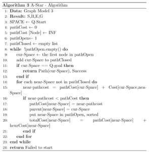
Algorithm 4.3. A-star algorithm, Created by Ryan Mbagna-Nanko based on information from Modern Robotics[2].
We maintain two lists: pathOpen and pathClosed
- pathOpen refers to the set of nodes that have been visited but not fully explored, meaning that their successors have not yet been examined. Essentially, this is a list of pending tasks.
- On the other hand, pathClosed refers to the set of nodes that have already been visited and fully explored, including the examination of their successors. These nodes have been added to the pathOpen list, if applicable.

Figure. 4.3. A-Star-algorithm illustration. Solved example made using GraphOnline, Created by Ryan Mbagna-Nanko based on information from Modern Robotics[3]
Solution
To solve the problem given above, the A-Star algorithm can be used to find the shortest path between the start node, S, and the end node, G. The algorithm would start at the S node and then explore its neighboring nodes to determine which one is the best to visit next. This process continues until the algorithm reaches the G node, at which point it returns the shortest path between the two nodes.
As a result, the optimal path is S,B,E,G. In a practical sense, this method is the best way for the mobile robot in a manufacturing plant to determine the shortest distance to its handler. Its heuristic function ensures both cost and distance from the goal allows for a shorter run-time and more optimal solution is found in real-time.
4.2.2 Sampling-based methods
A generic sampling method relies on a random or deterministic function to choose a sample from the workspace (Cfree). These functions categorize whether the sample is “free” and “closed” than the previous free-space sample. Next, a local planner tries to connect to, or move toward, the new sample from the previous sample. This process builds up a graph or tree representing possible routes for the robot. Sampling methods are easy to implement, and suitable for search problems with high dimension space. Though satisfactory, the solution is not always optimal, and the computational process can grow more complex [2].
Sampling-based planners use randomized techniques to plan a path between a start and goal configuration, without relying on a pre-defined search algorithm. The process involves generating a sequence of configurations using a random sampling strategy, typically from a uniform distribution across the configuration space. If two configurations are close enough, a local planner can be used to plan a path between them. Repeating this process leads to the creation of a graph, also called a roadmap, that represents the possible paths between the start and goal configurations [3].
This section describes two different planning algorithms that rely on sampling. The first algorithm is called a probabilistic roadmap (PRM), which is designed to cover the entire free configuration space evenly. This can be useful when multiple planning problems need to be solved for the same workspace, as it can save time and effort in building the roadmap. The second algorithm is called a rapidly-exploring random tree (RRT), which uses a smart approach to create new vertices in the tree. This technique has been successful in solving challenging path planning problems [3].
4.2.2.1 Probabilistic RoadMap Planner (PRM),
A probabilistic road map planner is an algorithm that helps to solve the challenge of identifying the route for a robot between its start and destination points while avoiding obstructions. This approach is most suitable for addressing motion planning problems with complex high-dimensional configuration spaces [2].
A probabilistic roadmap planner consists of two phases:
- Construction Phase: A graph is built, which can be made in the environment. First, a random configuration is created. Then, it is connected to some neighbors, typically either the k nearest neighbors or all neighbors less than some predetermined distance. Configurations and connections are added to the graph until the roadmap is complete enough to connect the start and goal.
- Query Phase: The start and goal configurations are connected to the graph, and the path is obtained by the A* query.
Algorithm 4.4. PRM algorithm, Created by Ryan Mbagna-Nanko based on information from Modern Robotics[2].
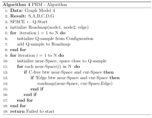
The graph given below represents a simple scenario in which a mobile robot needs to find the shortest path between its starting point, S, and its destination, G. The graph consists of several nodes and edges, with each node representing a specific location and each edge representing a path or connection between two nodes. In this case, the numbered nodes represent the potential obstacles in the environment, while the nodes with letters make up the graph. To solve this problem, let’s use the PRM algorithm for finding the shortest path between nodes S and G in the graph.
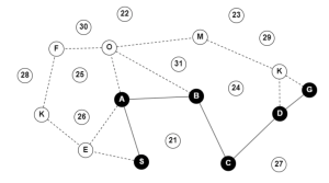
Figure. 4.4. PRM algorithm illustration. Solved example made using GraphOnline, Created by Ryan Mbagna-Nanko based on information from M.R. [3]
The process of constructing a Probabilistic Roadmap (PRM) can be described as relatively straightforward, as shown through the given pseudocode. A further breakdown is as follows. The first step involves generating a set of random configurations that serve as vertices in the roadmap. These configurations are typically generated uniformly across the free configuration space. The next step is to generate a set of paths that connect pairs of configurations in the roadmap. A simple local path planner is used for this task. The goal of this step is to create a roadmap that adequately covers the free configuration space [3], Fig 4.5, showcases this initial configuration, as the lettered nodes are scattered across the given space.
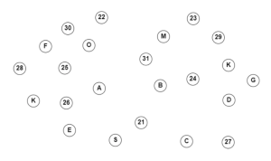
Figure. 4.5. PRM algorithm initial scattering of nodes. Example made using GraphOnline, Created by Ryan Mbagna-Nanko based on information from Modern Robotics [3]
Once the initial roadmap is generated, the algorithm checks if it consists of multiple connected components. If so, an enhancement phase is initiated, in which new vertices and edges are added to connect the disjoint components of the roadmap. This ensures that the entire free configuration space is covered and there are no unreachable areas.[3]
To solve a path planning problem, the PRM is used to connect the start and goal configurations, referred to as Qstart and Qgoal, respectively. The simple, local planner is used to add these configurations to the roadmap, and the resulting roadmap is searched to find a path from Qstart to Qgoal. Once a solution path is found, it is passed back to the simple, local planner, which refines the path to produce a final, optimized solution [3]. Fig 4.4, showcases this next phase, as the lettered nodes are connected across the given space.

Figure. 4.6. PRM algorithm connected nodes. Example made using GraphOnline, Created by Ryan Mbagna-Nanko based on information from Modern Robotics [3]
Solution
Overall, the PRM algorithm is designed to produce an efficient and effective roadmap that covers the free configuration space and can be used to find a collision-free path between the start and goal configurations. Once executed, the PRM algorithm returns S,A,B,C,D,G as demonstrated in Figure. 4.4. The use of PRMs allows the possibility of building a roadmap quickly and efficiently relative to constructing a roadmap using a high-resolution grid representation. In a practical sense, this method may help direct the mobile robot in a manufacturing plant to its handler. However, it does not necessarily consider the most cost-effective or shortest path to its desired goal.
4.2.2.2 Rapidly-exploring Random Tree (RRT)
As previously mentioned, one of the flaws of PRM is that there is no consideration on whether the path taken is the most cost-effective or shortest to its desired goal. As an alternative, another method is to grow a single tree, starting from the vertex corresponding to Qstart, until it reaches Qgoal. This approach is also known as rapidly-exploring random trees (RRT) [3]. The RRT algorithm begins by randomly generating points and connecting them to the closest existing node. Each time a new vertex is generated, it is verified to make sure it is not located within an obstacle. Furthermore, the new vertex must be linked to its nearest neighbor while avoiding any obstructions. The algorithm stops when a node is generated within the goal area or when a predefined limit is reached. RRT is a motion planning algorithm that considers robot kinematics/dynamics, but can be simplified by only considering its geometric approach.
Many factors that must be considered when applying the RRT algorithm [2].
- In this algorithm, we use a finite number of iterations. As the iteration number increases, we have more ways to move from start to goal.
- The tree generated should be inside the obstacle-free space Cfree of the configuration space we created.
- We also have a list that basically holds all the nodes which are part of the tree. This is created in order to check the closest node of the tree to the sampled random node created.

Algorithm 4.5. RRT algorithm, Created by Ryan Mbagna-Nanko based on information from Modern Robotics [2].
The terminology used in the pseudocode is introduced as follows:
- The map contains the map with obstacles. Nodes are generated in the roadmap by sampling in the configuration space.
- tree-MAX size is the maximum iteration for the RRT algorithm.
- Q-sample is the node generated by sampling, near-Space is the node that is near to the Q-sample and is already created in the configuration space.
- motion() is the function that is deployed by the local planner to move from Q-sample to Q-nearsample.
The process of constructing a Rapidly-exploring Random Tree (RRT) can be described as relatively straightforward, as shown through the given pseudocode. A further breakdown is as follows. Based on a starting point, we choose a random point in the space around the robot, called Q-sample. We find the closest point in the tree to the Q-sample, called the Q-nearsample node, and make that new point another starting point as cur-Space. By taking a step towards Q-sample from Q-nearsample node. We attach the cur-Space node to the Q-nearsample node and add an edge between them. We repeat these steps until we find the goal location or reach the maximum number of points allowed [3] [2].
The graph given below represents a simple scenario in which a mobile robot needs to find the shortest path between its starting point, S, and its destination, G. The graph consists of several nodes and edges, with each node representing a specific location and each edge representing a path or connection between two nodes. In this case, the numbered nodes represent the potential obstacles in the environment, while the nodes with letters make up the graph. To solve this problem, let’s use the RRT algorithm for finding the shortest path between nodes S and G in the graph
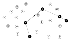
Figure. 4.7. RRT algorithm illustration. Solved example made using GraphOnline, Created by Ryan Mbagna-Nanko based on information from M.R. [2]
Solution
Overall, the RRT algorithm is an improvement from PRM. Once executed, the RRT algorithm returns S,A,M,K,G as seen in Fig 4.5. A significant gain in the RRT algorithm is seen in building a roadmap in the direction of its end point. In a practical sense, this method may be more effective in directing the mobile robot in a manufacturing plant to its handler. However, it does not necessarily consider the most cost-effective route, therefore not optimal.
Rapidly-exploring Random Tree (RRT) algorithms are known for their ability to plan paths that are free of collisions for robots. However, the true strength of these algorithms lies in their approach to generating and connecting new nodes, specifically Q-nearsample, to the existing tree. In contrast to Probabilistic Roadmap (PRM) algorithms, which connect new nodes by solving a local path planning problem, RRT algorithms select the configuration Q-nearsample by “taking a step” towards Q-sample. The simplest method is to move along a straight-line path towards Q-sample, but more advanced techniques can also be employed [3].
4.2.2.3 Rapidly-exploring Random Tree – Star (RRT*)
RRT* is an enhanced version of the RRT algorithm that is extensively used for solving robotics motion planning problems. The RRT* algorithm aims to provide the shortest path to the goal as the number of nodes approaches infinity. Although this goal is not practically feasible, the algorithm works towards developing a path that is as close to the shortest path as possible. All in all, RRT* is a robust and efficient algorithm that can find near-optimal solutions to challenging path-planning problems quickly [2].
- First, RRT* records the distance each vertex has traveled relative to its parent vertex. This is referred to as the cost of the vertex. After the closest node is found in the graph, a neighborhood of vertices in a fixed radius from the new node is examined. If a node with a cheaper cost than the proximal node is found, the cheaper node replaces the proximal node.
- The second difference RRT* adds is the rewiring of the tree. After a vertex has been connected to the cheapest neighbor, the neighbors are again examined. Neighbors are checked if being rewired to the newly added vertex will make their cost decrease. If the cost does indeed decrease, the neighbor is rewired to the newly added vertex.
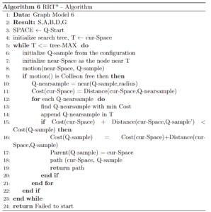
Algorithm 4.6. RRT-Star algorithm, Created by Ryan Mbagna-Nanko based on information from [7].
The terminology used in the pseudocode is explained as follows:
- The map contains the map with obstacles. Nodes are generated in the roadmap by sampling in the configuration space.
- Max.Treesize is the maximum iteration for the RRT* algorithm.
- Q-sample is the node generated by sampling, Q-nearsample is the node that is near to the Q-sample and is already created in the configuration space and Q-nearsample is the nearest node in Q-sample.
- motion() is the function that is deployed by the local planner to move from Q-sample to Q-nearsample
- near() is the function that finds all the nodes(Q-nearsample) from the Q-sample within the input radius.
The process of constructing a The process of constructing a Rapidly-exploring Random Tree – Star (RRT*) can be described as relatively straightforward, as shown through the given pseudocode. A further breakdown is as follows. The RRT* algorithm starts in the same way as the basic RRT algorithm, by initializing the tree with a single vertex representing the start configuration. A Q-sample is then randomly generated in the free configuration space, and the algorithm finds the Q-nearsample node in the existing tree that is closest to the Q-sample.
Instead of simply adding the cur-Space node as a child of the Q-near node, the RRT* algorithm first calculates the cost of the path from the start node to the Q-new node, and compares it to the cost of the path to the Q-near node plus the cost of moving from the Q-near node to the cur-Space node. If the cost of the new path is lower, the Q-new node is added as a child of the Q-nearsample node, and the cost of all affected nodes in the tree is updated to reflect the new path [7].
In addition, the RRT* algorithm iteratively rewires the tree by checking if any of the other nodes in the tree can be reached more efficiently by going through the new node. If a better path is found, the tree is rewired to reflect the new path, and the costs of all affected nodes are updated. This allows for a smoother path [7].
Here is an example: A mobile robot wants to calculate the shortest distance between the start, S, and the goal, G, while calculating a subpath which is also the shortest path between its source and destination. Given the graph below, use the RRT-Star method to determine the shortest distance traveled by the mobile robot to its destination.

Figure. 4.8. RRT-Star algorithm illustration. Solved example made using GraphOnline, Created by Ryan Mbagna-Nanko based on information from Modern Robotics. [2].
Examples
Overall, the RRT* the algorithm is an improvement from RRT. Once executed, the RRT algorithm returns S,A,B,D,G as seen in Fig 4.8. A significant gain in the RRT algorithm is seen in building a roadmap in the direction of its end point, while also considering “Cost-to-go”. In a practical sense, this method may be the most effective path planning method given a high resolution configuration. However, this method is limited by the resolution of the configuration space. This applies to most sampling methods, as the goal of such algorithms is to iteratively scan the configuration space. This can be further improved.
The primary distinction between RRT and RRT* is that RRT* employs a cost-to-go heuristic function, which estimates the distance to the goal from each node in the tree. This heuristic function guides the expansion of the tree towards the goal region, leading to a more efficient search for the optimal path [2].
Moreover, the rewiring of the tree edges during the algorithm is another significant difference between RRT and RRT*. In RRT*, the edges are continuously rewired to improve the optimality of the tree. This rewiring process involves searching for a better path between any pair of nodes and re-routing the tree if a better path is found [2].
4.3 Multiple Robot Design Setup
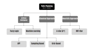
Figure. 4.9. Flowchart of Classification of mobile robots path planning approaches Created by Ryan Mbagna-Nanko based on information from [9]
Multi-Robot Path Planning covered can be categorized as classical or heuristic approaches. Classical approaches include APF and sampling-based algorithms, which require more time and space and may not ensure completeness. Heuristic approaches, like A*, are faster and more efficient in finding globally optimal paths using a cost function.

Figure. 4.10. Centralized decision making structure Created by Ryan Mbagna-Nanko based on information from [9]
An essential aspect of path planning for multiple robots is making decisions about task prioritization and queueing. While in series, Qgoal can be assigned in sequence, to operate multiple robots in parallel would require more attention to the structure of decision-making. Path planning is part of the multi-robot system’s consideration, and the structure of the multi-robot system can be classified as centralized or decentralized based on the planner. The multi-robot system is centralized if the system has supervisory control or a central planner. For robots making their decisions, the system is decentralized.
Figure. 4.11. Decentralized decision making structure Created by Ryan Mbagna-Nanko based on information from [9]
Multi-robot systems can be classified as centralized or decentralized based on the path planning approach used. Centralized systems (Figure 4.10) have a central planner that directly controls each robot, resulting in better control and task assignment. Classical, heuristic, and AI-based techniques are applicable, but they have limitations in dynamic situations. Decentralized systems (Figure 4.11), on the other hand, allow robots to communicate and share information, using various algorithms such as heuristic, optimization metaheuristic, neural networks, APF, and sampling-based approaches. Real-time updates and fault tolerance are crucial in decentralized systems to keep the system running and update the robot’s status. [9]
4.3.1 Simulation setup – Virtual Environment via python
In regards to collision avoidance, multi-robots should be able to adjust their defined task plans or paths in real-time to achieve the tasks if necessary. This has no limitations of the system framework for fault tolerance because the centralized framework can inform all robots quickly, and the decentralized framework can send the fault signs to the neighbor robots.
Given the scope of this chapter is limited as an introduction to path planning, the nature of the demonstrated experiment will showcase a centralized framework. In addition, our understanding of offline path planning and the classical methods is extended to multi-robot path planning in series. In this case, the mobile robots tasks / Qgoal is predetermined, and the path-planning method is applied in sequence. However, a more advanced heuristics approach as proposed in “FAULT-DETECTION ON MULTI-ROBOT PATH PLANNING”[10] would be a potential solution to control multiple mobile robots in parallel to their desired Qgoal.
The technical details for this experiment is as follows: We will rely on coppelia-sim as our simulation environment featuring a single “Pioneer 3-DX” as the robot to demonstrate each offline-path planning methods discussed. The next phase will be to feature two “Pioneer 3-DX” as the robot to demonstrate each offline-path planning in sequence. The set environment is featured in Fig 4.12. Each algorithm is programmed in python via Spyder. Therefore, Coppelia Sim is controlled remotely via “Remote API”. For more details check out the Github Repository. In the meantime, feel free to play around with these sample programs, and make it your own. Happy learning!
A simulation is done to showcase the goal to avoid obstacle using RRT Path Planning Method in Copplia-sim.

Figure. 4.12 Top view of the Coppelia-sim Simulation environment featuring single Pioneer 3-DX [left] two Pioneer 3-DX [Right]
Figure. 4.13 Top view of the Coppelia-sim Simulation environment featuring single Pioneer 3-DX with RRT Path Planning [left] two Pioneer 3-DX with RRT Path Planning [Right]
The coppliasim file and python script can be accessed through https://github.com//Ch4_Path_Planning
4.4 Summary
In today’s economy, manufacturing plants have grown to adopt logistics technology to modernize everywhere. By inviting collaboration in shared space between humans and robots, most industries have evolved to fulfill growing demand by optimizing planned paths taken by mobile robots in a given space. In this chapter, we demonstrate many properties to motion planning as it pertains to path planning. The various methods showcase application of multiple vs single query, and an understanding of completeness and computational complexity [3].
In a given space with obstacles, the Cspace is partitioned into Cfree (free space) and Cobs (obstacle space). Checking if a configuration is collision-free involves using a simplified representation of the robot and obstacles. To check if a path is collision-free, the individual configurations are sampled at closely spaced points. Based on the robot position and size, the path is checked for collision. The Cspace is often represented by a graph, with edges representing feasible paths, and nodes representing configurations. Edges can be weighted given their predicted cost. As a result, a solved path is mapped out from the Cfree, pointing the mobile robot from its starting point towards the end goal .
A grid-based path planner discretizes the Cspace into a graph consisting of neighboring nodes on a regular grid. The A* algorithm is the most popular search method. It operates by always exploring from a node that is (1) unexplored and (2) on a path with the minimum estimated total cost. Though Dijkstra and UCS are also suitable methods, they are often limited by the time it takes due to the lack of heuristic function. Overall, grid methods are easy to implement but only appropriate for low-dimensional spaces.
A sampling-based approach is suitable for high dimensional spaces. As discussed, PRM first maps out the entire space as a graph, ignoring the obstacles. A-Star then searches for the optimal path to the end goal. In a similar fashion, RRT forms a growing tree that fills the entire space. Occasionally, two trees are involved, one in the forward direction (Start to Goal) and in the backward direction (Goal to Start). However, this is not an optimal path-planning solution as the trees may not intersect, and there is no consideration of “Minimum-Cost”. This is later resolved via RRT-STAR.
In a space dominated by mobile robots and human personnel acting as the handle, path planning logistics are as important as the traffic signals in a busy city. Given the increased demands, it is expected that there will be both expected and unexpected obstacles in any manufacturing warehouse. Given that mobile robots each have their own role, and are required to be in certain spaces at a given time, it is imperative that the mobile robots make decisions and correctly plan their way around obstacles, nor become obstacles for others. Overall, manufacturing logistics ensures synchronization between each robot and the human handler, given the working environment.
4.5 Practice
1. What is the difference between Motion-Planning and Path Planning?
- Path Planning is an umbrella term, and Motion planning is a subset
- Motion Planning is an umbrella term, and Path planning is a subset
Ans: Motion planning is an umbrella term used in robotics for the process of breaking down the desired movement task into discrete motions that satisfy movement constraints and possibly optimize some aspect of the movement. Path Planning is a subset, focused on mapping routes to a desired end point, while avoiding obstacles along the way.
2. What is Grid-Based Motion Planning?
- In Grid-based, collision-free space is divided into smaller cells
- In Grid-based creates possible paths by randomly adding points to a tree until some solution is found
Ans: Grid-based motion planning is a technique, where the collision-free space is divided into smaller cells, where the graph node is at the center of the cell.
3. What is Sample-based Motion Planning?
- In Sample-based, collision-free space is divided into smaller cells
- In Sample-based creates possible paths by randomly adding points to a tree until some solution is found
Ans: Sampling-based algorithms represent the configuration space with a roadmap of sampled configurations. it creates possible paths by randomly adding points to a tree until some solution is found.
4. What is Configuration Space?
Ans: Configuration space is a collision-free space where the robot is able to move inside the path considering the robot’s dimensions.
5. Which is the most efficient grid-based motion planning algorithm and why?
- Dijkstra
- UCS
- A*
Ans: When I compared the three grid-based motion planning algorithms, the most efficient was A*because the heuristic helps choose the only nodes near the goal state.
6. Which is the most efficient sampling-based motion planning algorithm and why?
- PRM
- RRT
- RRT*
Ans: RRT and RRT* are very efficient compared to PRM planner because the PRM planner requires creating a graph and then we use A* for determining the shortest path, which is time-consuming and occupies huge storage.
7. [DIY Challenge] Can you write an RRT-Star planner for a physical mobile robot moving in a controlled space with obstacles. Given the image captured from a video camera, Free space and obstacles are represented by a two-dimensional array, where each element corresponds to a grid cell in the two-dimensional space.The occurrence of a 1 in an element of the array means that there is an obstacle there, and a 0 indicates that the cell is in freespace.Your program should plot the obstacles, the tree that is formed, and show the path that is found from the start to the goal. (Adapted from Modern Robotics [2])
4.6 Reference
[1] LaValle, S. M. (2014). Planning algorithms. Cambridge University Press.
[2] Kevin M. Lynch Modern Robotics: Mechanics, Planning, and Control, Jul 6th, 2017
[3] Mark W. Spong, Seth Hutchinson M. Vidyasagar. Robot Modeling and Control,
[4]Tyagi, Neelam. “What Is Dijkstra’s Algorithm? Examples and Applications of Dijkstra’s Algorithm.” What is Dijkstra’s Algorithm? Examples and Applications of Dijkstra’s Algorithm. Accessed from https://www.analyticssteps.com/blogs/dijkstras-algorithm-shortest-path-algorithm.
[5]“Uniform-Cost Search (Dijkstra for Large Graphs).” GeeksforGeeks. GeeksforGeeks, April 20, 2023. https://www.geeksforgeeks.org/uniform-cost-search-dijkstra-for-large-graphs/.
[6] Majetiha, Dipali. “Uniform Cost Search.” Medium. Medium, October 5, 2019. Accessed from https://medium.com/@dipalimajet/understanding-hintons-capsule-networks-c2b17cd358d7#:~:text=Uniform%20Cost%20Search%20is%20the,less%20the%20same%20in%20cost.
[7]Chinenov, Tim. “Robotic Path Planning: RRT and RRT*.” Medium. Medium, February 26, 2019. Accessed from https://theclassytim.medium.com/robotic-path-planning-rrt-and-rrt-212319121378.
[8] “Warehouse Robotics Market by Type, Payload Capacity, Application,, Offering, Industry Vertical – Global Opportunity Analysis and Industry Forecast, 2023–2030.” ReportLinker. Accessed from https://www.reportlinker.com/p06428925/Warehouse-Robotics-Market-by-Type-Payload-Capacity-Application-Offering-Industry-Vertical-Global-Opportunity-Analysis-and-Industry-Forecast.html?utm_source=GNW#summary.
[9] “A Review of Path-Planning Approaches for Multiple Mobile Robots”, Machines 2022 Accessed from https://www.mdpi.com/2075-1702/10/9/773
[10]Singh, Ashutosh Kumar, & Naveen Kumar. “FAULT-DETECTION ON MULTI-ROBOT PATH PLANNING.” International Journal of Advanced Research in Computer Science [Online], 8.8 (2017): 539-543. Web. 6 May. 2023
Additional Resources
- https://www.coursera.org/learn/modernrobotics-course4?specialization=modernrobotics#syllabus
- https://modernrobotics.northwestern.edu/nu-gm-book-resource/chapter-10-autoplay/#department
- https://graphonline.ru/en/#
- https://www.coppeliarobotics.com/helpFiles/en/zmqRemoteApiOverview.htm
