10.1. Introduction

In this chapter, we will briefly introduce the concepts surrounding Lie theory and how they may be applied to robotics applications in advanced manufacturing. We will introduce the idea behind smooth manifolds and then describe how they tie to Lie groups and Algebra. We will then discuss important properties related to Lie groups and how exploiting their smooth structure and diffeomorphism with Lie algebra allows us to work in the tangent space embedded in , a linear space more familiar to us for performing calculus and calculations.

This chapter introduces basic concepts regarding manifolds and differential geometry, enabling us to perform geometric control of mechanical systems. The advantages of working on a manifold structure as opposed to a Euclidean structure that we are familiar with are discussed. Lie theory, in general, is a very Mathematically heavy subject requiring a rigorous background in topology, differentiable geometry, and multivariable calculus. This chapter serves as a beginner-friendly introduction to basic concepts and their implications in the vast field of robotics.

The next two sections of this chapter will be focused on introductory theory regarding Lie algebra and its application in robotics for manufacturing.

10.2. Basic Concepts in Lie theory

This section will explain various concepts that will help us form some basic intuition behind how Lie theory can be utilized for robotics applications. Note that Lie theory requires vast prerequisite knowledge to understand its intricacies. However, we will be introducing basic concepts regarding Lie theory. We will focus on inculcating a general understanding of the advantages of working with Lie theory and how they translate into robotics.

10.2.1. Smooth Manifolds

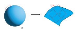
Generally, a manifold can intuitively be understood as a generalization of curves and surfaces to higher dimensions; an example is shown in Figure 10.1.

Created by Aayush Rai based on information from [1]

To give a more precise definition, a real n-dimensional manifold   is a topological space that is homeomorphic to the Euclidean space at each point. In simple terms, this means that a manifold locally resembles the Euclidean space near each point. That is, if you zoom in enough on a manifold, the underlying structure will appear to be in .

Created by Aayush Rai based on information from [1]

Throughout this chapter, we will only be concerned with smooth manifolds. As the name implies smooth manifolds can be quite simply visualized as surfaces and shapes embedded in higher dimensions that have no ‘edges’ or discontinuities. In order to transfer over the concepts of calculus such as differentiation and integration or solving ODE  ’s (Ordinary Differential Equations) which are vital to the field of robotics, we require some notion of ‘smoothness’. The main reason for this is that a smooth manifold that can be projected into locally would enable us to perform all such calculations and to define smooth functions in the curved space itself. The smooth structure of a manifold also implies the existence of a unique tangent space at each point which will be discussed later.

An example of a smooth manifold can be a 3-Dimensional sphere which may be locally approximated to as shown in Figure 10.2. So in this particular case, one basic thing to keep in mind is that intuitively, one would like to say that the sphere is a 3-dimensional manifold but that would be wrong, look back on the definition and remember that the dimension of a manifold is determined by the dimension of that it looks like locally, so a sphere is a 2-dimensional manifold. Similarly, let’s consider a circle as a manifold, since locally, it is embedded in (looks like a line locally), it is a 1-dimensional manifold.

Another way to look at manifolds is that it describes or is defined by the constraints on the state. For example, vectors with the unit norm constraint define a spherical manifold of radius one.

Discussion on the underlying topology of smooth manifolds is omitted here, the reader can refer to [1] for a more rigorous discussion.

10.2.2. Lie theory

The mathematician Sophus Lie (LEE) initiated lines of study of Lie theory [19] and discovered that the continuous groups (Lie groups) could be better understood by linearizing them and studying the corresponding vector fields which is called the Lie algebra.

Lie theory is concerned with the study of Lie groups which are high-dimensional smooth manifolds with a group topology. The tangent space of these groups is a linear space that encapsulate all the information about the group itself.  Such a tangent space evaluated at the ‘identity’ elements of the group is called the Lie algebra of the group. As we will see in later sections, the tangent space of a Lie group evaluated at identity has a nice linear structure with some nice properties that enable us to identify Lie group elements by its Lie algebra. (Note: for now, you can think of the ‘identity’ element of a group as something when multiplied by an element of a group returns the group element itself.)

10.2.3 Lie Groups

A Lie group   is defined as a smooth manifold that also satisfies the group properties. Let us review the group axioms briefly.

A group is a set with a composition operation   that, for elements satisfies the following axioms.

A Lie group is characterized by a unique identity element and the two group operations of multiplication and inversion:

(10.2)

where .

Let us look at what these properties mean. The first property of equation (10.2)   says that the composition of two elements of the Lie group stays within the group itself and the second property says that all elements within the Lie group have an inverse that is also within the group itself. Also, all Lie groups have an identity element. Without diving too deep into the topology of sets themselves, what we can understand from this is that if we have a set of elements that satisfy the group axioms in equation (10.1) and Lie group properties given in equation (10.2), the set itself is endowed with a ‘smooth’ structure [1].

Let us consider an example of a common Lie group that are frequently used in robotics, i.e., the Special Orthogonal group of rotations.

(10.3)

Elements of this group are called rotation matrices and this group encompasses all possible 3-D rotations. As the name of the group suggests, elements of this group are orthogonal with determinant equal to one. It is easy to verify that rotation matrices satisfy properties given in equation (10.1) and equation (10.2) imposed by the group structure. We know by composition of rotations that the multiplication of two rotation matrices also gives us a rotation matrix and that their inverses exist and are also rotation matrices. Also, the ‘identity’ element of this group is the 3X3 identity matrix . Since from eq (10.3), we can see that , and for rotation matrices, we know that , hence the inverse property associated to the identity element of the group is satisfied as well.

Some of the applications of rotation matrices are [2]:

• Multiplication by a rotation matrix can change the orientation of a vector.
• A rotation matrix by itself also represents a position.
• A base reference frame can be multiplied by a rotation matrix to get a new frame.

Another common Lie group used in robotics is the Special Euclidean group . Elements of this group are called the homogenous transformation matrices and they map rigid body motions.

(10.4)

This group encapsulates rotation as well as translation of a rigid body as opposed to just rotation which we just saw for . Here, the rotation matrix accounts for the rotation of the rigid body and comprises of the values of the displacement of the rigid body. The application of these matrices is similar to rotation matrices, only instead of just rotation, translation plus rotation takes place.

Throughout this chapter, we will be focusing on these two Lie groups that are very prominent in robotics namely the group of rotations and the group of rigid body motions. All the concepts covered from here will be explained on either of these two Lie groups.

10.2.4. Lie group action

In this section, we will discuss how Lie groups can transform other sets to perform rotations, translations etc. We will give a formal definition first and then illustrate this using examples.

Given a Lie group and a set , we note the action of on ,

Here represents the action between the Lie group and the set . It is defined as a mapping from to , which means that when a Lie group action is performed on an element of a set , then the result is also an element in which has been appropriately transformed.

For to be a group action, it must satisfy the following axioms,

1) Identity: , where is the identity element of the group.
2) Compatibility:

Let us see how this action takes place using and Lie groups:

: rotation matrix
: Euclidean matrix

In the first case, the vector is rotated through the action of the Lie group on it and in the second case, the vector is rotated and translated by the action of the Lie group on it.

10.2.5. Tangent Space and the Lie Algebra

The main advantage of Lie theory is that a curved object such as a Lie group can be identified by its linear tangent space at the identity [3]. Note that whenever we talk about the tangent space , the subscript refers to the point on the manifold at which the tangent space is evaluated. As mentioned before, a manifold being smooth such as the ones endowed with a group structure (Lie groups) have a unique tangent space at each point and their structure remains the same at all points as well. Because they have a unique tangent space at each point, we can accurately map back and forth between the tangent space and the group without worrying about uniqueness, also since the underlying structure remains the same, we are able to work on the linear tangent space which has the same dimension everywhere throughout the manifold. Now we are starting to build some intuition on why it is always smooth manifolds that we are interested in.

Created by Aayush Rai based on information from [5]

The Lie algebra of a Lie group is defined as its tangent space at the identity. The tangent space of a Lie group at the identity consists of the tangent vectors to smooth paths in where they pass through .

Note: ‘ ‘ here refers to the identity element of the group.

Let us consider a path in , it is called smooth if the time derivative exists and if , we call the tangent or velocity vector of at.

Let us derive the Lie algebra for matrix Lie groups. As discussed before, tangent space elements at 1 of a group are matrices of the form.

where is a smooth path in with , which means that the path is passing through at time . Tangent vectors can be viewed as velocity vectors of points moving smoothly through the point of the group. Let’s take a simple example of an matrix, i.e., consider a Lie group of 2-D rotations as follows:

(10.5)

This matrix represents a smooth path through since . The derivative of the matrix gives us

The corresponding tangent vector at will be

Let us look at what this means geometrically. This means that all tangent vectors at the identity form the 1-dimensional vector space of real multiples of the matrix . What this means is that any point on the tangent space of the manifold with respect to the identity element can be recognized by multiplying with and this Lie algebra element can be mapped back into the group by taking its matrix exponential which will be introduced later.

Another important thing to remember is that the dimension of the tangent space of a manifold is always equal to the dimension of the manifold itself.

Created by Aayush Rai based on information from [5]

This makes sense since we know that the manifold is the group of 2-D rotations represented by a circle which is a 1-dimension manifold embedded in 2 dimensions. Recall our definition of manifolds, their dimension is determined by the dimension of the Euclidean space they are homeomorphic to. Since in this case, we can see that locally, the circle will look like a line embedded in , so its tangent space will also be embedded in as well, which means a straight line basically. The tangent space of at will be a line as can be seen in figure 10.4. We can also get some sense of the identity element of a group through the figure, here the identity element e corresponds to a 0 degree 2-D rotation and as we move along the circle, the value of will change and so will the group elements and the corresponding tangent space, as shown in figure 10.4 for some arbitrary point . So, substituting in equation (10.5), we can get the identity element of the group as the 2X2 identity matrix.

Note that this is a very basic example of a very simple manifold to motivate the understanding of the concept of the identity element of a group and its corresponding tangent space so that they can be thought of in an abstract sense and not necessarily in the context of trivial manifolds.

We are now able to discuss the tangent space of and its corresponding Lie algebra. Before we do that, lets formally define as a group.

The rotation group in -dimensional Euclidean space, , is a continuous group, and can be defined as the set of by matrices satisfying the relations [4]:

We know that represents the 3-dimensional rotation group. Similarly, we can think of as an -dimensional rotation group that rotates planes at once.

We know that for satisfies . Let be a smooth path originating from

(10.6)

Taking the derivative of equation (10.6), we get

(10.7)

For , substituting in equation (10.7), we get

(10.8)

So, any tangent vector that satisfies is part of the tangent space at identity.

The matrices that satisfies equation (10.8) are skew symmetric since we have .

Now, let’s look back to elementary calculus from which we know that for any commuting variables and .

What’s remarkable is that the matrices and appearing in the condition we have for the tangent space of matrices, i.e., , also commute. This means that we can identify the elements of the Lie group from its Lie algebra by taking the matrix exponential of the skew symmetric matrices.

Also, we can show that is an orthogonal matrix as expected because

To summarize, what we have derived just now is that the tangent space for matrices are skew-symmetric matrices which can also be mapped back as group elements by taking the matrix exponential of these matrices [3].

Consider an example of a rotation matrix representing the 3-D group of rotations, so we have

(10.9)

Taking the derivative of Equation (10.9), we get

From this, we can infer that is a skew-5ymmetric matrix [5], now for , we get and

(10.10)

where is the vector of angular velocities. The tangent space of at identity is denoted by (also called the Lie algebra of ) whose elements are skew-symmetric matrices.

10.2.6. Generators of Lie Groups

We will directly illustrate generators of Lie groups through an example on . Intuitively, we can think of generators of a Lie group as the basis of the corresponding Lie algebra.

Let us look back at the skew-symmetric matrix for the Lie algebra of in equation (10.10)

The generators of correspond to the derivatives of rotation around each of the standard axes evaluated at the identity [11]. The corresponding generators are

These can be seen as the decomposition of the Lie algebra matrix.
Elements of can be expressed as a linear combination of generators (hence the ‘basis’ intuition)

(10.11)

Looking back on the tangent space, recall how it just had 1 generator

10.2.7. Lie Bracket

An important concept that must be introduced regarding Lie theory is that of the Lie bracket. The motivation to work on the tangent space of a Lie group is that we can infer all the associated properties of the group from the linear space. Lie algebra is the vector space tangent to the identity together with an antisymmetric and bilinear operator called the Lie bracket. As we saw in the previous section, exponentiation of the tangent space gives us the elements in the group.

Not all Lie groups are necessarily commutative and this property can be captured by the tangent space as well with the help of Lie brackets. We can also say that the Lie bracket monitors the lack of commutativity in multiplication.

If and are matrices in the tangent space, then the Lie bracket is defined as [10]:

(10.12)

It is also a property of Lie groups that the Lie bracket of matrices in the Lie algebra is also in the Lie algebra.

Let us illustrate this concept through a simple example, is an abelian group and hence its Lie bracket will be zero since they are commutative groups, this means that for these groups

which then implies that and makes the Lie bracket zero. A commutative group operation on is completely captured by the sum operation on the tangent space [3]

Now consider the group of rotations, we know that this group is not abelian, i.e., intuitively we know that if we rotate a rigid body through its axis followed by a rotation through axis, we will end up with a different orientation when the order of rotations is reversed. For such groups, we will have

10.2.8. Exponential and Logarithmic map

The exponential and logarithmic maps are used to map back and forth between Lie groups and their tangent space as shown in figure 10.5. Geometrically, what this means is that the exponential map wraps the tangent vector around the manifold like wrapping string around a ball and the curved path made by this string is called the geodesic [5]. The inverse of this operation is the unwrapping of this string embedded in a linear space.

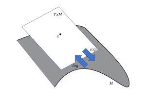
Created by Aayush Rai based on information from [5]

This concept is visually shown in Figure 10.6. Note that the tangent space is at and not at the identity. We will now illustrate this concept using the group.

Created by Aayush Rai based on information from [5]

As we have seen previously, the derivative of a rotation matrix can be written as

(10.13)

Again, note that since is in multiplication with , it belongs to the tangent space at and not at the identity. The solution to equation (10.13) is given by

(10.14)

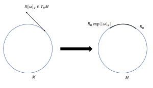
where is the element of the Lie group from where the curve begins, i.e., identity as shown in figure 10.6. Before we proceed further, let us look at equation (10.14) and correlate it to Figure 10.6. As varies from 0 to 1 , we can see that varies from to which encapsulates the ‘wrapping’ concept we introduced earlier, i.e., the exponential map gives us a curve that smoothly varies from whichever point we consider the tangent space on to the point given by the multiplication of the initial element of the Lie group and the exponential map of the Lie algebra element.
At the identity , the solution is given by

(10.15)

We now define the vector as the integrated rotation in the angle-axis form, with angle and unit axis . Thus, is the total rotation expressed in the Lie algebra. We substitute it into equation (10.15) and write the exponential as a power series [5],

We omit the proof and directly state the Rodrigues formula [5] for matrix exponential for

(10.16)

The exponential map yields a rotation of radians about the axis given by .
The logarithmic map going from to is given by

(10.17)

10.2.9. Baker Campbell Hausdorff (BCH) formula

For and in the Lie algebra, the BCH formula is defined as the solution to for equation (10.18) given as

(10.18)

The formula asserts that can be written purely in Lie algebraic terms [12] (Lie bracket).

What we can intuitively infer from this is that the Lie bracket on the Lie algebra determines the product operation on . There might be some cases where we need to find explicitly and this formula might come in handy. This is also a fundamental formula that is used to prove some important proofs in Lie theory which are beyond our scope for now.

10.2.10. Hat and Vee map

We can go from the Lie algebra to with the help of isomorphisms called hat and vee which are defined as follows [5]:

Hat : Vee :     (10.19)

where are the generators of the Lie algebra and are the vectors of the base . In general, when dealing with adjoints and Jacobians on Lie groups, it is much easier to work in the space and vectors in this space are isomorphic to the Lie algebra, so information about the group is not lost as well.

10.3. APPLICATIONS TO ROBOTICS IN ADVANCED MANUFACTURING

Lie theory has a wide range of applications in the field of robotics. Taking advantage of the smooth manifold structure of the Lie group in tandem with the Linear tangent space is the fundamental motivation behind these applications.

Some applications include optimization on manifolds, rigid body attitude control by formulating system kinematics and dynamics on a Lie group, state estimation and Kalman filtering and many others. In this section however, we will be focused on Lie group methods that aid manufacturing applications.

10.3.1. SCREW THEORY

Screw theory helps us to easily formulate the kinematics and dynamics of multi-body systems such as manipulators that may be used for manufacturing purposes. It also improves efficiency of computational algorithms on multi-body systems [13]. In the case of continuum robots which find extensive use in manufacturing applications, screw theory provided a more intuitive way of parametrizing curves and surfaces [21]. Jacobian calculation for multi-fingered robots is also made easier using screw theory [20].

Screw theory is a powerful mathematical tool for analysis and formulation of multibody kinematics. A screw can be used to denote the linear and angular velocity of a rigid body.

Created by Aayush Rai based on information from [6]

Have a look at figure 10.7, an alternate way of thinking of a transformation matrix is via what’s called a Screw. Think of a Screw as a stick attached to the back of an object like a link or joint. You can turn the screw about its axis to rotate the end object by angle of and you can move the screw around to translate the object ). The pitch defined in the figure is the amount of linear motion for a given rotation, which means,

• Pitch accounts for pure rotation
• Pitch accounts for pure translation

A screw is defined by a unit direction axis , the position of a point on this axis with respect to a reference frame and pitch .

(10.20)

Zero pitch screws which correspond do pure rotation where are given by

Infinite pitch screws corresponding to pure translation motion where are given by

We state these explicitly since they correspond to revolute and prismatic joints which are seen frequently in open kinematic chains.

We will now state Chasle’s theorem for twist.

The most general motion of a rigid body consists of a rotation about a line in space together with a translation along it. Such a quantity is called twist or spatial velocity [6].

(10.21)

Now that we have defined the notion of a screw, a twist can be interpreted in terms of this screw and a velocity about it. A twist represents the velocity of a rigid body as the angular velocity about an axis and the linear velocity along an axis. The expression for the twist is given by .

Recall that we defined the group previously as one that encompasses all rigid body motions. We will now see how this group relates to the screw coordinates defined above. First, let’s define the Lie algebra of the group. The Lie algebra is the set of matrices corresponding to differential translations and rotations. An arbitrary element in is given by

Where is the skew-symmetric matrix of angular velocities and v represents the linear velocity.

Let denote the screw coordinates. The matrix exponential is defined as then for any distance traveled along the screw axis or any angle rotated about the screw axis [6],

(10.22)

where,

Which we know from the Rodrigues formula defined previously in equation (10.16)
If and , then

(10.23)

The proof of this is omitted but the main takeaway here is that exponentiating the screw coordinates, we get an matrix that represents rigid motions. Keep in mind that we are exponentiating and not , here represents the Lie algebra element in as defined above corresponding to the screw coordinate .

(10.24)

where is the skew-symmetric matrix of angular velocities and represents the linear velocity.

This should come as no surprise since we have shown in previous sections how taking the exponential of elements in Lie algebra gives us the corresponding Lie group elements, the only difference here is in terms of representation, we are using screw coordinates to construct an matrix and then taking its exponential.

Now, let’s introduce an important concept that will help us in formulating the forward kinematics of kinematic chains.

Given the position of the end-effector of the kinematic chain in base frame, its forward kinematics can be computed using the product of exponentials formula as [6]:

(10.25)

where represents the screw coordinates of the joint expressed in the base frame and is the respective joint displacement.

This basically means that we simply need to find the screw coordinates of each joint in the base frame in order to calculate the forward kinematics. We can express the screw coordinates in , take their matrix exponential and multiply them to get the result.

Example 10.3.1.1.

Let’s consider a simple example of a 2-D case to showcase how screw theory works for multi-link manipulators.
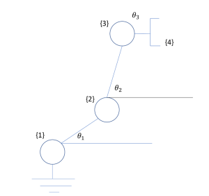
Consider the 3-link system given below in figure 10.8 .

Created by Aayush Rai based on information from [6]

 

Look back on the definition of screw coordinates defined in equation (10.20), we will now define and for all three links and their associated [6].

We know that since all three joints are revolute and , since rotation is always along the axis.

For link 1,
For link 2,
For link 3,

The corresponding screw coordinates $S$ for these links can be calculated from equation (10.20) as

Now, we can go ahead and calculate the corresponding matrices as given in equation (10.24), note that when we perform this step, we always assume screw coordinates to be for the form .

The zero pose configuration of the end effector is given by

By the product of exponentials formula given in equation (10.25), we can write the forward kinematics as

Now that we have a general understanding of how screw theory works, we are now able to evaluate why this method of computing forward kinematics is superior to other existing methods.

An important observation that can be made regarding screw theory is that everything is formulated in the base frame of reference, this contrasts with Renayit-Hartenberg parameters where we must introduce different reference frames for each joint. Not only does screw theory simplify kinematic modeling but a lot of algorithms on such multi-body systems depend on the way the kinematics are defined. The computational algorithms defined on such system become more efficient when the underlying kinematics are defined using screw and Lie theory. [13]

10.2.2. Computer Vision

Lie theory has extensive applications in computer vision [22], motivated readers can refer to this research paper [7] for further discussion on its applications. Industrial cameras can be used in the manufacturing space for precise robot control for pick and place operations, for example, a robot gripper with a 3-D camera module. They are also used to inspect components and track movements of robots used for manufacturing. Motivated by such applications, we will now introduce how Lie theory can be used in parallel with computer vision.

We will be considering the concept of Rotation averaging in this section. Rotation averaging is important in the field of computer vision, visual data can be given as a sequence of 3-D rotations [9] which may contain a lot of noise and require smoothing. Another important application of rotation averaging is in the case of camera-rig calibration [8]. The rotation averaging techniques discussed in both the papers will be discussed in this section with focus on how they showcase the capabilities of Lie theory.

First, let us go ahead and define the distance metric on .

A distance measure is called bi-invariant if

for all . This is just a formal definition of a bi-invariant metric, we do not necessarily need to focus on it for now. We can now define the angular distance metric between rotations. [9]

Any rotation in can be expressed as a rotation through a given angle about some axis. We define the angular distance between two rotations and to be the angle of the rotation , so chosen to lie in this range .[9] Thus,

where the norm is the usual Euclidean norm in and .

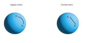
There is also a chordal metric on which is visually shown coupled with the angular metric in figure 10.9.

Created by Aayush Rai based on information from [9]

What we can infer from this is that the angular metric is geometrically ‘nicer’ since elements on the line traced by this matrix also lie on the manifold itself which is not the case for the chordal metric. So, as a motivation, suppose we perform some calculations involving the angular metric, the result will still be a rotation matrix which is what we generally desire whereas for a chordal metric, this will not be the case.

We will now formally define the Karcher mean of rotations on a manifold and then introduce the same on the manifold.

Let be a set of points in a smooth Riemannian manifold . The Riemannian metric can then be used to obtain the geometric distance between any two points . The Karcher mean of this set is defined as the point for which the sum of squared distances [9]

(10.26)

is minimized. A necessary and sufficient condition for to be the Karcher mean is

The iterative algorithm for computing this mean is given as [9]

1. Set initial mean in as .
2. Compute the mean in as .
3. While , update to ( , for and go to step 2

Where is some small tolerance value. Let’s analyze this algorithm. First, we pick any arbitrary point from our set to be the initial mean, we then use the logarithmic map to calculate the mean on the tangent space centered around this point, and if this mean is above the tolerance limit, we update our initial mean using the exponential map to move towards the point where the mean is being minimized.

As discussed, let’s consider the Karcher mean for the group of rotations to get a better idea of how the algorithm works visually. The rotation minimizing

(10.27)

is also known at the Karcher mean of the rotations. A necessary and sufficient condition for to minimize this function is given by

(10.28)

What this means geometrically is that if is the mean of rotations, then when it is mapped to the tangent space, it is equidistant from all other rotation matrices in the sense that the positive and negative ‘distances’ between these elements cancels out.

The iterative algorithm is given by

1. Set initial mean in as .
2. Compute the mean in tangent space of centered at as .
3. While , update to , and go to step 2

Visual representation of this algorithm is given in figure 10.10.

Created by Aayush Rai based on information from [9]

As shown in figure 10.10 , we first select , center the tangent space around this element and map all the other elements onto this tangent space, we then calculate the mean which is shown by the green dot and then map it back to the manifold and use it as an updated mean to repeat the process on its tangent space. When the mean calculated on the tangent space is sufficiently close to the element we centered the tangent space on, we say that the algorithm has converged and we have found the Karcher mean.

Another rotation averaging technique that is more robust to outlying errors is the L1 rotation averaging with Weiszfeld step on the manifold. We will not discuss this method in detail in this section, interested readers may refer to [9] for a more comprehensive discussion. In contrast to the metric used in L2 rotation averaging given in equation (10.27), the metric used for rotation averaging, as the name implies is

(10.29)

Where is the angular metric for the distance between the two rotation matrices. This method is similar to other methods in the sense that it takes advantage of the linear structure of the tangent space to perform calculations. The main idea here is that we are familiar with performing gradient descent on a linear space, when that underlying space is changed to , we take advantage of the linear structure of its tangent space to perform gradient descent and then map back to the manifold using the exponential map. Weiszfeld step provides away for us to perform gradient descent in a closed loop fashion, since it gives us an analytic formulation for the step size. [18] A step-by-step roadmap of how this takes place is given as follows:

1. Take as an initial mean (preferably the average)
2. Apply the logarithmic map centered on for all other elements
3. Calculate the Weiszfeld step on the manifold: this tells us which direction we must go towards in order to minimize the metric given in equation (10.29)
4. Use the exponential map to apply the calculated step on the manifold.
5. Repeat steps 1 to 4 until convergence

10.2.3. Rigid Body Control

Control of rigid bodies is an essential aspect for robots used in manufacturing applications such as UGV’s (Unmanned Ground Vehicles), UAV’s (Unmanned Aerial Vehicles), manipulators and many others. There is extensive literature on geometric methods (using manifold theory and differential geometry) being used for attitude control. [14,15,16] We will be focusing on rigid body tracking on $S O(3)[16]$ in this section, the reader may refer to the paper cited for a detailed explanation. Even though some of the concepts employed in the paper have not been covered in this chapter, we will focus more on an intuitive understanding on how rigid body tracking may take place on a manifold.

We will focus on deriving control laws using functions on . Now, a question may be asked regarding why we want to define our problem on a manifold. Using geometric control techniques, which basically means by formulating our research problem on the manifold itself instead of taking its linear approximation, allows for the formulation of a coordinate free control system. This enables us to define a geometric control system that has several advantages over traditional control such as avoiding gimbal lock [16].

We will be considering a first order system as compared to the second order system presented in [16] to formulate the control law. Let’s consider the pose of a rigid body given by the rotation matrix and let be the rotation matrix associated to the trajectory that we are supposed to track. Let and be the associated skew symmetric matrices in . The system kinematics will be given as

Here, we assume that all information regarding will be known to us and we wish to formulate control laws for the input which is a skew-symmetric matrix of yaw, pitch and roll angular velocities.

The desired controller of the rigid body should satisfy rigid body tracking given as

(10.32)

where is the Frobenius norm. It basically gives a measure of the rotation required to align and , we can logically think of it as an error that we eventually want to converge to zero. A detailed explanation on how this condition accounts for the domain in is given in [16], for now, let’s just think of this as our tracking goal.

The paper introduces a function family that induces a controller class. These functions depend on and . The conditions for a function to be in this family of functions is omitted here but the reader may refer to [16] for a detailed analysis.

Let be a function on the family , taking the Lie derivative [1] of this function along the vector fields given by equation (10.30) and equation (10.31), we get

(10.33)

Now, let us consider a real valued positive definite Lyapunov function defined as

(10.34)

where represents the square of the 2-norm of the vee mapping as we defined previously in equation (10.19)
Taking the derivative of equation (10.34), we get

(10.35)

The required condition to make negative definite is given as

(10.36)

Substituting the derivative of defined in equation (10.33), we get

(10.37)

Hence, for the derivative of the Lyapunov function to be negative definite, we get

(10.38)

The controller for is then given by

(10.39)

This controller will ensure that the Lyapunov function given in equation (10.34) converges to zero since it makes the derivative negative definite. This means that if we select a suitable function for our purposes, we should be able to formulate a controller for rigid body tracking on .

Let us consider the function

(10.40)

as given in [16] for rigid body tracking. First, we need to define the derivative of this function for us to substitute it into equation (10.36) to get our required control law.

First, let us consider $R_d(t)^{\top} R(t)$, the derivative of this is given as [16]

(10.41)

Keep in mind that the time derivative of defined in equation (10.40) is defined in the usual form that we are familiar with as defined in the previous section in equation (10.13), which is as the multiplication between the rotation matrix itself and its associated skew-symmetric matrix.

Now, let’s derive what the time derivative of the logarithmic map of a rotation matrix will look like. We know that a rotation matrix can be expressed as

(10.42)

as we have seen previously in equation (10.14). Taking Log of both sides, we get

(10.43)

Taking the time derivative of equation (10.43), we get

What we can infer from this is that the derivative of the logarithmic map of a rotation matrix is equal to the associated skew symmetric matrix of that rotation matrix in . From equation (10.41), we know the associated skew symmetric rotation matrix associated to , so the time derivative of given in equation (10.40) is given as

(10.44)

Replacing this in equation (10.36), we get

Equating the terms in the vee map, we get

(10.45)

Equation (10.45) gives us the control law for the skew-symmetric matrix for the yaw, pitch and roll angular velocities of the rigid body that tracks a desired trajectory .

10.4. Summary

In chapter 10, we introduced the concept of Lie theory by introducing smooth manifolds and Lie groups. The main advantage of working with Lie groups is that we can work in its tangent space which is a linear space and allows us more freedom to do calculations. Moreover, the group structure itself is captured by its corresponding Lie algebra and we can map back and forth between the Lie group and its tangent space using the exponential and logarithmic maps. Lie algebras are characterized by an additional metric called the Lie bracket which allows us to monitor the anti-commutative structure of the group.

We first give a brief description of smooth manifolds and then go on to define Lie groups and introduce two of the most common Lie groups used in robotics which are the Special Orthogonal group and the Special Euclidean group . The tangent space and Lie algebra of Lie groups is discussed and we particularly focus on and show that its Lie algebra is given by the skew-symmetric matrix given in equation (10.10). The next section of the chapter discusses different characteristics of Lie group such as the exponential and logarithmic map to map back and forth between the manifolds, we introduce the concept of generators of a Lie group, hat and vee map between Lie algebra and the Euclidean space as given in equation (10.19). Although its applications are not discussed, we define the Lie bracket on the Lie algebra and show how they measure the non-abelian nature of the Lie group, we then showcase the significance of Lie bracket through the Baker-Campbell-Hausdorff (BCH) formula.

Moving onto the manufacturing applications of Lie theory, we showcase how it may be used to define and understand screw theory which is a simplified way to define the forward kinematics of multi-link robotic manipulators. We also explain how Lie theory may be used in the field of computer vision with particular focus on rotation averaging on the manifolds. Finally, we introduce how Lie theory may be used for rigid body control and why its beneficial to formulate functions on the manifold space as opposed to the Euclidean space.

 Practice Problems

1. Prove the Rodrigues’ formula given in equation (10.16) using the Taylor series expansion.

 

Answer. We can write the rotation matrix R(t) as

where is the integrated rotation in angle-axis form, with angle
and unit axis and is the lie algebra matrix of angular velocities.

Expanding, we get

Let us first write down a few powers of

As we can see, all powers can be expressed in terms of , and . We can write the Taylor series expansion as

Now, we can identify the Taylor series expansions of and and write the Rodrigues’ formula as

 

2. Based on your intuition from the 2D case, how do you think you might interpolate the rotations using the exp/log map for 3D rotations?

We can just do the same thing: given two rotations $R_0$ and $R_1$, the rotation between them (in axis-angle form) i.e.  is given by

Hence, we can interpolate via

As before, this family of rotations starts at $t=0$ with $R_0$, and interpolates to $R_1$ at $t=1$.

 

3. Show and explain why gimbal lock would occur by calculating the rotation matrix  .

Consider the matrix given by and extract the roll, pitch and yaw angles of the resulting rotation matrix to confirm gimbal lock.

Answer.  

Using trigonometric identities:

Hence, when the pitch angle , the roll cannot be distinguished from yaw .

Calculating

Extracting the roll, pitch and yaw angles, we get 

which are totally different values than expected, hence confirming gimbal lock.

 

Simulations

The simulation utilizing concepts of Lie theory for computer vision and rigid body control can be found on GitHub at:

https://github.com/ClemsonSpring2023ME8930IntroRoboticsHRI/Ch10_Lie_Theory

References

[1]  Lee, John M. “Introduction to Smooth Manifolds.” Changes (2007).

[2]  Mark Saroufim “How to move? Lie Robotics” URL: https://marksaroufim.medium.com/how-to-move-lie-group-robotics-67fc4f3959d1

[3]  Stillwell, John. Naive lie theory. Springer Science & Business Media, 2008.

[4] Tyler Perlman. “Representations of the Rotation Groups ” URL: https://www.pas.rochester.edu/assets/pdf/undergraduate/representations_of_the_rotation_groups_so-n.pdf

[5] Sola, Joan, Jeremie Deray, and Dinesh Atchuthan. “A micro Lie theory for state estimation in robotics.” arXiv preprint arXiv:1812.01537 (2018).

[6] Shivesh Kumar. “ Lie group based modelling of robot kinematics & dynamics and
An optimization based view on robotics” URL: http://www.stardust-network.eu/wp-content/uploads/2021/03/Shivesh_Kumar_Lie-group-based-modelling-of-robot-kinematics-dynamics.pdf

[7] Xu, Qiang, and Dengwu Ma. “Applications of Lie groups and Lie algebra to computer vision: A brief survey.” In 2012 International Conference on Systems and Informatics (ICSAI2012), pp. 2024-2029. IEEE, 2012.

[8] Dai, Yuchao, Jochen Trumpf, Hongdong Li, Nick Barnes, and Richard Hartley. “Rotation averaging with application to camera-rig calibration.” In Computer Vision–ACCV 2009: 9th Asian Conference on Computer Vision, Xi’an, September 23-27, 2009, Revised Selected Papers, Part II 9, pp. 335-346. Springer Berlin Heidelberg, 2010.

[9] Hartley, Richard, Jochen Trumpf, Yuchao Dai, and Hongdong Li. “Rotation averaging.” International journal of computer vision 103 (2013): 267-305.

[10] Tom Drummond “Lie groups, Lie algebras, projective geometry and optimization for 3D Geometry, Engineering and Computer Vision” URL: https://www.dropbox.com/s/5y3tvypzps59s29/3DGeometry.pdf?dl=0

[11] Ethan Eade “Lie Groups for 2D and 3D Transformations” URL: https://ethaneade.com/lie.pdf

[12] URL : https://en.wikipedia.org/wiki/Baker%E2%80%93Campbell%E2%80%93Hausdorff_formula

[13] Müller, Andreas. “Screw and Lie group theory in multibody kinematics: Motion representation and recursive kinematics of tree-topology systems.” Multibody System Dynamics 43, no. 1 (2018): 37-70.

[14] Yu, Yun, Shuo Yang, Mingxi Wang, Cheng Li, and Zexiang Li. “High performance full attitude control of a quadrotor on SO (3).” In 2015 IEEE International Conference on Robotics and Automation (ICRA), pp. 1698-1703. IEEE, 2015.

[15] Lee, Taeyoung. “Geometric control of quadrotor UAVs transporting a cable-suspended rigid body.” IEEE Transactions on Control Systems Technology 26, no. 1 (2017): 255-264.

[16] Akhtar, Adeel, and Steven L. Waslander. “Controller class for rigid body tracking on $\mathsf {SO}(3) $.” IEEE Transactions on Automatic Control 66, no. 5 (2020): 2234-2241.

[17] Mellinger, Daniel, and Vijay Kumar. “Minimum snap trajectory generation and control for quadrotors.” In 2011 IEEE international conference on robotics and automation, pp. 2520-2525. IEEE, 2011.

[18] Hartley, Richard, Khurrum Aftab, and Jochen Trumpf. “L1 rotation averaging using the Weiszfeld algorithm.” In CVPR 2011, pp. 3041-3048. IEEE, 2011.

[19] Lewis, Andrew D. “Is it worth learning differential geometric methods for modeling and control of mechanical systems?.” Robotica 25, no. 6 (2007): 765-777.

[20] Li, Zexiang, and S. Shankar Sastry. “Task-oriented optimal grasping by multifingered robot hands.” IEEE Journal on Robotics and Automation 4, no. 1 (1988): 32-44.

[21] Bajo, Andrea, and Nabil Simaan. “Kinematics-based detection and localization of contacts along multisegment continuum robots.” IEEE Transactions on Robotics 28, no. 2 (2011): 291-302.

[22] Lui, Yui Man. “Advances in matrix manifolds for computer vision.” Image and Vision Computing 30, no. 6-7 (2012): 380-388.

[23] URL: https://brilliant.org/wiki/abelian-group/