
7 Are Continuum Robots the Future of Advanced Manufacturing?
Nithesh Kumar
Are Continuum Robots the Future of Advanced Manufacturing?
7.1. Introduction
7.2. Design of Continuum Robots
7.2.1. Basic Design and Actuation principles of Continuum Robots
7.3. Modelling Continuum Robots
7.3.1. Robot Kinematics
7.4. Control Methods
7.5. Applications of Continuum Robots
7.6. Summary
7.7. Practice Questions
7.8. Simulations
References
7.1 Introduction
In this chapter we will take an in-depth look at continuum robots, their kinematics and their applications, and why they are primed for advanced manufacturing applications. Robotics in general is a vast field with major inroads being made every day. Robots have been around since the early 1950s and have progressively improved in complexity, functionality and productivity. Modern robots can be categorized by their varying sizes, dexterity and functionality. Robots can be classified into a myriad of categories, however, the simplest way to classify robots would be to distinguish them based on their functionality. Robots can be classified into two main categories based on the aforementioned classification: industrial robots and service robots. As the name suggests, industrial robots are most commonly used in commercial settings such as factories for manufacturing and assembly. Service robots are robots that aid humans in performing useful tasks. The ISO (International Organization for Standardization) defines such robots as “robots in personal use or professional use that performs useful tasks for humans or equipment”. Medical robots, home robots, entertainment robots, and agricultural robots are a few examples of such robots. Robots can also be classified based on their kinematics, i.e., their movement or lack thereof. Stationary robots are generally classified into the following categories, Cartesian, SCARA, cylindrical, spherical, articulated, wheeled or legged, airborne and aquatic etc.
Continuum robots fall under the category of stationary robots. A continuum robot is defined as a continuously bending actuatable structure, with one extremity fixed to a base. Continuum robots have an infinite degree of freedom (DoFs). With major advances being made in the field, continuum robots have been developed for a wide range of applications, such as manufacturing, aerospace, search and rescue, and some breakthroughs have been made on potential medical applications. In such scenarios, the infinite DoFs and the dexterity of these robots enable them to maneuver tight spaces that cannot be accessed by conventional robots with high precision. In this chapter we will delve into the basic design of continuum robots, the theory for modelling continuum robots, existing control strategies and their kinematics.
7.2 Design of Continuum Robots
7.2.1 Basic Design and Actuation Principles of Continuum Robots
In this section of this chapter, we take a more in-depth look at the basic design and actuation principle behind continuum robots. The foremost element behind continuum robots is their backbones. The backbone acts as the main structural component and facilitates bending as well as providing the basic shape of the robot itself. The primary issue that needs to be tackled in continuum robot design is the actuation of the backbone, i.e., how does one bend, extend and or contract the backbone? There are two basic design strategies that are most common in the design of continuum robots, extrinsic actuation and intrinsic actuation. These basic design principles are further discussed in the following sections.
Extrinsic Actuation
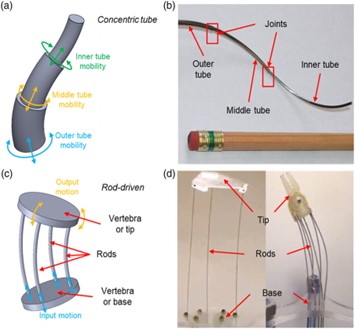
Extrinsic actuation is a design approach wherein the actuators are separate from the backbone and outside of the robot workspace. Generally, the actuation is generated at the base, and is then propagated through the backbone to generate the required bend/actuation. The placement of the actuators outside of the workspace provides a unique advantage in that this allows the backbone design to be simplified. Continuum robots with extrinsic actuation can be classified based on their actuation techniques. The two most common actuation techniques for extrinsically actuated continuum robots are tendon-driven continuum robots and concentric tube continuum robots. Tendon-driven continuum robots are actuated with sets of tendons routed along the backbone (Fig. 7.1). Groups of tendons are terminated at specific points along the backbone. When actuated, these tendons combine to bend the backbone to produce a series of sections, these sections generally tend to have constant curvature. The tendons bend a backbone that is nominally straight. Generally, tendon-driven continuum robots have a single continuous backbone, and the vertebrae of these robots act as a path for tendon routing, In the case of continuum robots with segmented backbones, the backbones also double up as structural elements. A constant curvature can only be approximated in continuum robots with a segmented backbone. The segmented backbones are made of various flexible elements between rigid bodies, such as hinges, compliant hinges and coil springs, which can also be used to control segment extension.

“Figure 1” by Matteo Russo et.al. is licensed under CC BY 4.0 / A derivative from the original work
Concentric tube continuum robots, also referred to as ‘active cannulas’ are made of pre-curved tubes nested inside of each other. The shape generated by the robot is controlled by translating and rotating each tube. The axial rotation and translation that enables the tubes to be inserted and retracted is provided by actuators present at the base of each pre-curved tube. This allows the tubes to intact elastically with each other, allowing the user to generate the desired bend and shape. These nested pre-curved tubes are of decreasing radius and increasing length. The tubes can also be rotated to give 2n degrees of freedom for an n-tube backbone. Concentric tube continuum robots have the smallest outer diameters out of all the continuum robots, which makes them suited for surgical applications. However, the two independent motors required for each actuator makes it a difficult design to upscale as the robot control is affected by structural elastic instabilities. However, recently, promising alternative designs with helical pre-curvature or patterned tubes improve performance, as well as hybrid designs with features from both tendon-driven robots and concentric tube robots have been developed and may, in fact, enable the use of such robots in medical and surgical applications.
“Figure 2” by Matteo Russo et.al. is licensed under CC BY 4.0 / A derivative from the original work
Intrinsic Actuation
Unlike extrinsic actuation, intrinsic actuation is a design approach wherein the actuators are within the continuum backbone. The majority of intrinsically actuated continuum robots comprise of backbones that are largely formed by their actuators. Continuum robots designed with intrinsic actuation technique uniquely provide the user with direct local control over the backbone shape, thereby providing the user with the ability to produce extensible backbones. Artificial muscle technologies such as pneumatic McKibben muscles, are most commonly used in continuum robots, and have proved most effective in the design of such robots, though other techniques such as shape-memory alloys (SMAs), dielectric actuators, and other similar materials can also be used for the same. The major disadvantage of using this actuation technique is that the onboard actuation renders the robot bulky, thereby making them not conducive for small scale applications. However, when compared to extrinsically actuated robots, intrinsically actuated robots provide a better force transmission efficiency, and therefore can potentially handle higher payloads, and the modeling and control of these robots are simplified compared to their extrinsically actuated counterparts.
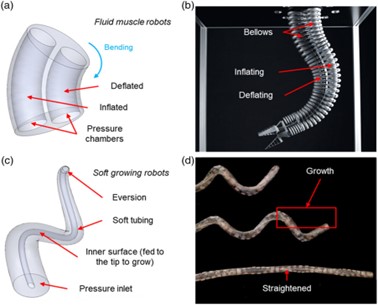
As mentioned before, while there is abundant active research on smart material actuators for use in intrinsically actuated continuum robots, pneumatics has been the most successful and most used design technique. The two main pneumatic designs that are widely used are fluid muscle-based robots, where the intrinsic actuation is achieved by using pressurized fluids in antagonistic soft chambers (Fig.7.3) and soft growing robots that increase in length when intrinsically actuated with pneumatics (Fig. 7.3 (c,d)).
“Figure 3” by Matteo Russo et.al. is licensed under CC BY 4.0 / A derivative from the original work
Scientists have been researching fluid muscle robots for nearly three decades. These types of robots are categorized by both continuous and segmented backbones. These robots are designed based on and behave similarly to antagonistic muscles. An antagonistic muscle pair is a pair of muscles in which one muscle contracts and the other muscle relaxes or lengthens. These fluid muscle robots are designed with pressurized chambers that inflate and deflate alternatively, which results in the desired backbone bend. As previously mentioned, these robots have a relatively high payload which makes them suitable for manipulation tasks in environments that are not very structured.
Soft-growing robots are unique and innovative in that they are designed by combining the flexibility of continuum robots along with the additional capacity to significantly extend their backbone. Growth is achieved by using a soft tubing folded into itself (Fig. 7.3 (c,d)), this in turn results in a pressurized inlet between its external surfaces (generally fixed at the base) and its internal surfaces (free to translate). When the pressure is increased in the inlet, a section of the internal surface unfolds at the tip with an eversion motion (outward or away from the robot), which results in the surface becoming the external surface and thereby increasing the total length of the robot. While this increase in length renders these robots ideal for long-reach applications such as search and rescue, they have some drawbacks such as low accuracy, payload, and motion controllability.
7.3 Modeling Continuum Robots
We can mathematically represent the behavior of continuum robots by modeling their kinematics. Robot kinematics is defined as the set of positions that entirely describes the system geometry based on the system and material mechanics such as governing equations, and constitutive laws respectively. In theory, a continuous flexible backbone features an infinite number of degrees of freedom. The traditional modeling techniques for robotics were designed for a finite number of serial rigid links and are no longer applicable. As discussed in the previous section, continuum manipulators feature a finite number of actuators, these actuators apply finite forces to the backbone at fixed, preselected locations therefore resulting in a significant increase in complexity when it comes to analyzing them. In this section, we take an in-depth look at the recent development of continuum manipulator kinematics.
“Figure 4” by Matteo Russo et.al. is licensed under CC BY 4.0 / A derivative from the original work
7.3.1 Robot Kinematics
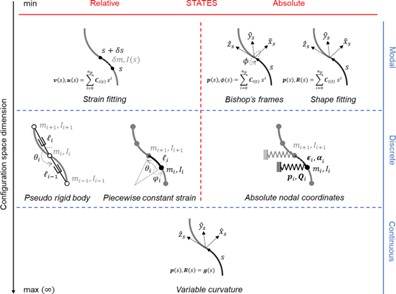
As previously mentioned in this section, the lack of distinct links in continuum robots makes the prevailing robot modeling techniques unsuitable. We can either model the backbone as a series of discrete elements or as one continuous differentiable curve (Fig. 7.4). Therefore, as a result of the continuous kinematic representations, we end up with a series of partial differential equations with differential states for the system’s equation of motion categorized as follows; Variable Curvature models, Modal techniques and the discrete (piecewise) kinematics approach. These are further discussed in the subsequent subsections.

“Figure 5” by Matteo Russo et.al. is licensed under CC BY 4.0 / A derivative from the original work
Discrete Kinematics
The discrete (piecewise) kinematics approach, while not as accurate as the continuous modeling techniques, provides us with an approximation of robot kinematics with discrete rods, pseudo rigid bodies (PRB), or other such elements. This technique enables us to take the kinematic models and control techniques used for standard rigid-body systems and apply them to continuum designs. The discrete techniques include the following: PRB kinematics where the backbone is modeled as a highly articulated rigid chain. This method approximates the robot backbone as a highly articulated rigid-body chain with elastic rotational and translational joints. Piecewise constant strain (PCS) is a technique where the local strains act as the relative states. The very common and widely used Piecewise Constant Curvature (PCC) method is a special case of PCS method where barring bending all the other states such as elongation, shear, and torsion are set to zero. The PCC model represents the system as a series of constant curvature elements, in this technique, the system kinematics is derived by either employing equivalent elastic joints or discretizing Variable Curvature (VC) relations. And finally, the absolute nodal coordinate formulation (ANCF) is a technique where the absolute nodal coordinates, both position and orientation are the system states. In simple words, this is a technique that divides the body of the robot into many discrete nodes. This method employs a Finite Element Modeling (commonly referred to as FEM) like framework in which techniques such as cubic polynomial fitting can be exploited to derive the element strain from the absolute states. The individual element kinematics can be represented by a shape function representation, such as constant curvature or a cubic polynomial curve by both PCS and the ANCF techniques.
Piecewise Constant Curvature (PCC) Method
While various models for continuum robots have been proposed, constant curvature assumptions are most commonly used due to their simplicity and the abundance of literature. Constant curvature is rarely observed due to several factors such as external and body loads, torsional strains, tendon friction, material behavior and a hoard of other issues. However, by discretizing the backbone curve into multiple constant curvature segments with relative or absolute states we can approximate a variable backbone curvature.
The PCC approach models the shape of a continuum robot with a series of circular arcs with constant curvature in space but variable curvature in time. As per Fig. 7.5a, each arc is defined by three independent variables, which describe the arc length (l), the bending angle given by θ, and the direction of bending which is given by φ. The resulting curve is characterized by a continuous differential, i.e., at their shared ends, the consecutive segments share the same tangent which depicts the robot’s backbone. The cross-section of the robot is usually assumed to be rigid and normal to the tangent of the backbone.
The base of the robot is defined by frame {S0} , a fixed orthonormal basis. The terminal vertebra of the ith segment is defined by frame {Si}. Equation (7.1) describes the transformation![]() from frame {Si-1} to {Si}. Here,
from frame {Si-1} to {Si}. Here, ![]() is the rotation and
is the rotation and ![]() is the translation along the arc which describes the segment.
is the translation along the arc which describes the segment.

As shown in Fig 7.5, when the motion is parameterized by bending direction (φ) and bending angle (θ), the rotation from frame {Si-1} to {Si} is given by the following,

And the translation can be written as, here is the is the length of the backbone from frame {Si-1} to {Si} The major limitation of this model is a kinematic singularity. In scenarios where any segment of the robot is in straight, i.e., θ = 0 Eq. (7.3) cannot be defined. This discontinuity, however, is a mathematical artifact caused by the model. Different parametrizations can sidestep this issue and alternatively, singularity-free modal approaches can also be used. While this section covers the PCC method in the context of modelling continuum robots, you will find a more detailed derivation on this approach applied to the modeling of soft robots in Chapter 8.
Absolute Nodal Coordinate Formulation (ANCF)
In Piecewise Constant Curvature discretization, sequential segments are related through compliant joints which move according to local strains on them. In ANCF kinematics, the nodes are defined with their Cartesian position and quaternion representation of orientation as the system’s absolute states. An element’s local linear strain (shear and elongation) and bending/twist angle vector ![]() are calculated based on the inverse map depicted in Eq. (7.4) and Eq. (7.5) which are in turn used to compute the system deformation energy. This map is obtained by linearizing the inverse Variable Curvature kinematics of a curve.
are calculated based on the inverse map depicted in Eq. (7.4) and Eq. (7.5) which are in turn used to compute the system deformation energy. This map is obtained by linearizing the inverse Variable Curvature kinematics of a curve.
 Here, Qi is the element’s absolute orientation quaternion, and Pi is the element’s position vector, × and * are the quaternion multiplication and rotation of a vector respective and defined in [3, 4]. ANCF is more conducive for modeling 1D elements such as continuum rods, as FEM mainly relies on the deformation of a 3D position field to detect changes in orientation. Both PCC and ANCF kinematics result in a finite-dimension system that facilitates the use of rigid-body techniques for nonlinear controller design and dynamic system analysis. On the contrary, geometrically exact modeling reproduces the exact deformation nonlinearity with no approximation to kinematic variables, usually relies on differential Variable Curvature with an infinite number of states.
Variable Curvature Models
Variable curvature models are based on continuous modeling technique, and provide an exact formulation based on a continuum mechanics model of system energy with infinite dimensional and a continuous configuration space. A couple of examples of such continuum mechanics models are Cosserat and Euler–Bernoulli rod/beam theories.
Variable Curvature kinematics With Cosserat Rod Theory
VC kinematics with the Cosserat rod theory illustrates the configuration of a flexible rod as a framed curve (Fig. 7.5b). In this section we will assess this theory in the context of modelling continuum robots, Chapter 8 dives deeper into the Cosserat rod theory as well as the and Euler–Bernoulli rod/beam theory extensive detail in the context of soft robotics. A Cosserat rod is defined by its centerline, which is the spatial curve of its mass centroid![]() In its initial configuration the curve is arc length parametrized, giving us
In its initial configuration the curve is arc length parametrized, giving us ![]() , where p’(s) is defined as the tangent vector at parameter value s, defined as,
, where p’(s) is defined as the tangent vector at parameter value s, defined as, ![]() and the curve length is given by the following equation:
and the curve length is given by the following equation:

The Cosserat rod theory assumes a rigid cross section of the rod, which is not necessarily normal to the tangent of the centerline curve. A frame can be defined based on the following equation,
 This frame can be used to describe the orientation of the cross sections along the rod. This enables us to model a continuum system as a ‘parametrized homogeneous rigid-body transformation’
 ![]() , with the cross-section orientation
, with the cross-section orientation ![]() and the center line position
and the center line position ![]() with respect to arc length s as follows,
with respect to arc length s as follows,
 The variables v(s), and u(s) can be used to represent the linear and angular rates of change respectively. The following equation aids in mapping out the evolution of g(s) along the arc length s, here
 ![]() is the representation of the transformation of vector u(s) into the space
is the representation of the transformation of vector u(s) into the space ![]() , specifically into SO(3) which is a skew-symmetric matrix, while the tangent unit vector at the base which is used to define the rod’s initial direction is given by
, specifically into SO(3) which is a skew-symmetric matrix, while the tangent unit vector at the base which is used to define the rod’s initial direction is given by ![]() , here the direction is along the global frame z-axis.
, here the direction is along the global frame z-axis.
 The Cosserat rod theory provides a geometrically exact model for continuum robots. However, it is more complex, and can be more computationally expensive than some of the techniques that we will be discussing in the subsequent subsections of this chapter.
Modal Techniques
Modal techniques (reduced-order model—ROM) provides a shape function which is based on the approximation of factors such as robot backbone shape, strain or cross-section geometry deformation using shape-fitting techniques such as cubic spline, Bezier etc. or a weighted sum of differentiable shape functions. This results in a differentiable finite state-space system which benefits from conventional modeling and techniques used for rigid-body systems.
The system differential kinematics is interpolated by a continuous curve, the new state spaces are the curve control parameters i.e., the fitting and modal coefficients and control point positions. The shape functions can act as the standard basis of a polynomial, a Taylor expansion power series, a Lagrange polynomial, a Fourier series etc. As Eq. 7.10 depicts, the general shape of a continuum rod, g(s), commonly expressed via a polynomial fitting of order np . Here Ci(t) is the time variant coefficient vector, which represents the system shapes and is the basis function (i.e., the polynomial shape). Power and spectral series as well as the modal approximations of the system kinematics have the same form as the following Equation, the only difference being that the time-variant coefficients are replaced by the modal participation coefficients, while the shape function is substituted by the system dominant deformation mode shapes.
The following equation is used to derive the system deformation energy, the relations that are interpolated from the robot orientation are differentiated based on an inverse map obtained from Eq. (7.9), allowing us to derive curvature u and the local linear strains v, as depicted in Eq. (7.11) and Eq. (7.12) respectively.
 However, the strain interpolated relations need to be integrated as represented in Eq. (7.9), to derive the local position p, matrix representation of rotation R required to calculating the inertial and external load actions such as the Coriolis forces.
We are presented with a reduced order representation of the system state space as result of shape of curvature fitting techniques. Strain fitting is favored for handling the internal forces such as tendon or pressure actuation, the differentiation steps involved in the shape fitting technique tend to be computationally expensive and are prone to singularities in inverse formulations. Whereas shape fitting is favored in situations where the constraints, external loads, inertial terms, and control objectives in task space exist. However, the drawback being that once again the technique can be computationally intensive as the integration involves some inaccurate approximations or implementation of numerical integration schemes. In the following section we will take a brief look at the control methods involved in controlling continuum robots and what some of the challenges are in trying to do so.
7.4 Control Methods
When it comes down to controlling continuum robots, we face a set of additional challenges when compared to standard rigid link robots. Characteristics such as their virtually infinite DOF motion, and their non–linear material properties impede the development of a unified control framework. We can classify the existing control methods by their modeling approach. There are three common control methods, model-based controllers, model-free controllers with data-driven techniques such as machine learning and empirical methods, and finally hybrid controllers, a combination of the two. In the model-based control approach, up to three kinematic models can link the robot’s four operating spaces. The operating spaces are listed as follows; actuation, monitored with the aid of encoders and wrench sensors, joints (tendon length), configuration (shape parameters), and task space, i.e., the cartesian position and orientation of the end effector. Low-level controllers can be implemented in to track and compensate for actuator and/or joint-related errors such as cable friction, tendon coupling, and hysteresis. The configuration and task space controllers act directly on the robot’s motion target, providing a solution to model uncertainties, and making the performance more stable and robust. As a side note however, the actuator/joint space controllers are more stable and allow for higher frequencies with better dynamic performance. On the contrary, the model-free approaches are independent of joint and configuration parameters, and therefore can provide a more stable performance in situations where either the environment is unstructured or the system is highly non-linear, situations where model-based approaches tend to falter. Though, model-based controllers tend to be more reliable when compared to their model-free counterparts and are favored in critical applications such as medical and surgical robots. In the subsequent section, we will explore some of the applications of continuum robots.
7.5 Applications of Continuum Robots
In this section of the chapter, we will assess some of the current applications of continuum robots and how they might potentially translate to the manufacturing industry. A “natural” application for continuum robots is in the medical field. Medical applications have been a primary driving factor for continuum robot research. Substantial progress has been made in design, modeling, control, sensing, and application to specific medical problems and extensive reviews for this application exist [5,6]. The small size and compliance of continuum robots is very advantageous from a medical point of view. However, this places high demands on sensing, control, and human–machine interaction. Two teleoperated continuum robot systems, from Hansen Medical Inc. and Stereotaxis Inc., and one teleoperated hyper-redundant system from Medrobotics Inc. have obtained FDA clearance and are now commercially available. It is very likely that over the next decade will see continuum robots increasingly aiding surgeons and patients alike by providing less invasive access pathways and manipulation possibilities.
As discussed at the beginning of this chapter, Continuum robots are ideal for applications requiring higher malleability to the non-ideal environment. This ability of such continuum systems to maneuver tight congested environments makes them suitable for application areas beyond the scope of traditional robots. Recently there have been major developments in research behind using continuum robots for aerospace applications, most notably, using aeroengine repair. A 1.2-meter-long continuum robot with a tip with a 15mm diameter was the first robot demonstrated for industrial ever industrial aerospace application. The robot is fitted with two cameras and grinding tools at the tip that are interchangeable. The robot can uniquely navigate tight spaces in order to access an aeroengine from the front to inspect and repair low-pressure compressors. A continuum robot with five degrees of freedom which was operated remotely was used in teleoperates aero foil repair. A five-meter-long continuum robot with a 9.1 mm diameter was utilized in the inspection and maintenance of an aero engine. In another demonstration of their versatility in aerospace applications, a pair of 0.7 -meter-long continuum robot arms independently manipulated realized a thermal barrier coating repair of a commercial aeroengine combustor. The robot arm pair manipulated an extreme temperature flame of 3000 °C to successfully implement the necessary repair. While there haven’t been many major breakthroughs yet in terms the research behind continuum robots for manufacturing applications, the inspection and repair techniques we just discussed have the potential to be either scaled down or replicated and used in manufacturing settings such as vehicle or spacecraft manufacturing and/or assembly. Specifically, either in assembly of intricate parts, or potentially in scenarios which require high temperature tolerance such as welding or molding or in part inspection. In other words, scenarios that might require navigating otherwise tight and/or spaces inaccessible, potentially making it easier for the manufacturer to identify and fix any issues that may persist in such areas.
The unique flexible backbone of continuum robots aids them in conforming to objects of any shape, therefore enabling a “gentle” grasp on easy-to-damage objects such as fruit and vegetables, or items with complex geometries and a variety of object classes, due to their ability to adapt their shape to interact with the environment through non-local continuum contact conditions. Continuum manipulators, hands and grippers with continuum fingers etc., have been discussed in the literature on soft robotics and are recently subjected to studies to obtain grasp taxonomy which will potentially aid in the synthesis and control of grasping operations with continuum robots. Breakthroughs in this area are likely to lead to new designs and applications for the manufacturing setting. Continuum robots with such dexterity and flexibility potentially combined with robust grasping could help cut down on manufacturing time by aiding in the assembly of intricate parts. However, the challenge of designing such a continuum robot with both precision control and hardware design that would allow such flexibility remains.
Continuum robots are starting to become more common, there is a vast amount of research going into designing, developing, modelling and controlling continuum robots. While they are currently scarce in the manufacturing industry, they have the potential to be very useful in such settings. The continued research into continuum robots will only hasten the development of such robots for use in the manufacturing sector and it is not outrageous to believe that in a decade, such continuum robots will be a mainstay on the manufacturing floor.
7.6 Summary
In this chapter we took an in-depth look at continuum robots. We delved into the basic design of continuum robots, where we covered the basic design and actuation principles behind continuum robots, we also looked at some of the theory behind modeling and controlling continuum robots, their kinematics, as well as some their applications. Despite the substantial body of work and progress in the field, it is prudent to note that the research behind continuum robots remains in its early stages, many significant questions and issues remain open ended.
Newer and wider applications for continuum robots are necessary for the field to continue to thrive and grow. Applications in medicine nurtured the field is currently, and is likely to remain, a key focus of interest and research in the area. Nonetheless, industrial, and more specifically the manufacturing interest is ever growing, as continuum robots are uniquely designed to be capable of on-site inspection, maintenance, and repair tasks on infrastructures that might not be easily accessible to traditional rigid-link robots. As discussed, in this chapter, the application focus of continuum robots is widening. The catalyst to inspire both new ideas and current research to grow the field to match its vast potential is the identification and pursuit of new, and unique applications for such robots. The main purpose of this chapter is to provide the reader with some basic knowledge and understanding of continuum robots, and hopefully inspire and aid them to continue researching the subject matter.
7.7 Practice Questions
(Q 7.1) What is the simplest way of classifying robots?
ANS: Robots can be classified into two main categories industrial robots and service robots. As the name suggests, industrial robots are most commonly used in commercial settings such as factories for manufacturing and assembly. Service robots are robots that aid humans in performing useful tasks. The ISO (International Organization for Standardization) defines such robots as a “robot in personal use or professional use that performs useful tasks for humans or equipment”.
(Q 7.2) What is the definition of a continuum robot?
ANS: A continuum robot is defined as a continuously bending actuatable structure, with one extremity fixed to a base.
(Q 7.3) How many Degrees of freedom do continuum robots have?
ANS: Continuum robots have an infinite degree of freedom (DoFs).
(Q 7.4) What are some of the advantages of continuum robots compared to conventional robots?
ANS: The infinite DoFs and the dexterity of these robots enable them to maneuver tight spaces that cannot be accessed by conventional robots with high precision.
(Q 7.5) What are the two basic design strategies involved in designing continuum robots?
ANS: The two basic design strategies that are most common in the design of continuum robots are extrinsic actuation and intrinsic actuation.
(Q 7.6) What are the differences between extrinsically actuated and intrinsically actuated continuum robots?
ANS: Extrinsic actuation is a design approach wherein the actuators are separate from the backbone and outside of the robot workspace, whereas, intrinsic actuation is a design approach wherein the actuators are within the continuum backbone.
(Q 7.7) What is the drawback of using the Cosserat rod theory to model continuum robots?
ANS: The Cosserat rod theory provides a geometrically exact model for continuum robots. However, it is more complex, and can be more computationally expensive than some of the techniques that were discussed in this chapter.
(Q 7.8) What are variable curvature models?
ANS: Variable curvature models are based on continuous modeling technique, and provide an exact formulation based on a continuum mechanics model of system energy with infinite dimensional and a continuous configuration space.
(Q 7.9) How does one classify the existing control methods for continuum robots?
ANS: We can classify the existing control methods by their modeling approach. There are three common control methods, model-based controllers, model-free controllers with data-driven techniques such as machine learning and empirical methods, and finally hybrid controllers, a combination of the two techniques.
(Q 7.10) What are some of the applications of continuum robots?
ANS: Some common applications of continuum robots include, surgery, hazardous operations such as bomb disposal, nuclear site actions, maintenance, space craft maintenance and repair etc.
7.8 Simulations
The research behind modeling and simulating continuum robots is in its early stages and we are a fair way from being able to model and simulate continuum robots like we do with their rigid link counter parts. The goal of understanding the effects of tendon routing friction on the shape of continuum robots has been one that has driven the efforts of numerous research groups. Such groups modeled the tendon–vertebra interaction in given robot designs. Even such groups proved that the shape of the robot is influenced by and then modeled it with good accuracy they are limited by factors such as simplifications and lumped parameters, while in general being challenging to implement. Modeling continuum robots results in a system of nonlinear algebraic equations in the case of discrete kinematic and static models, an ordinary differential equation for modal and discrete dynamic models or partial differential equations for modal static and Cosserat rod models. Direct forward integration schemes such as Runge–Kutta can be used for ODEs in the absence of loads, or in a general case with known base wrench or in dynamic derivation based on discretized kinematics such as PCC. Else, a root finding or a boundary value problem will be formed to be solved by indirect numerical schemes such as shooting which relies on Jacobian-based numerical optimization, FEM solvers, or Ritz and Ritz–Galerkin methods. Developing software frameworks for modeling and control of continuum robots is garnering attention, and a number of research groups are working on addressing the needs of the growing multidisciplinary continuum robotic research community.
For the purposes of this chapter, we will be looking at SoRoSim (Soft Robot Simulator) a user-friendly MATLAB toolbox that is designed based on the Geometric Variable Strain (GVS) approach to provide a unified framework for the modeling, analysis, and control of soft, rigid, and hybrid robots. The toolbox can be used to analyze open, closed, and branched structures as well as allowing the user to model several different external loading and actuation scenarios. Simply put, SoRoSim, is a MATLAB toolbox that directly extends rigid robot modeling techniques to soft and hybrid systems whilst maintaining a high level of accuracy. This toolbox takes advantage of the high fidelity of the Cosserat rod approach and the simplifying assumptions of the GVS approach that minimize the number of DoF required to represent the system and provide a geometrically exact framework. This lends to accurate, fast, and computationally less expensive results.
SoRoSim allows the user to define and manipulate robotic systems (linkages) as well as links, both rigid and soft links alike using user-friendly GUIs and the MATLAB workspace. The GUIs aid in the definition of links, the assembly, and the definition of the DoF of the defined links, the assignment of constraints as closed-loop joints, and the application of external and actuation forces. The GUIs can handle a variety of typical external forces and actuation inputs, this provides a black-box experience, allowing users from varied backgrounds and experience to easily use the toolbox to perform static and dynamic analysis. The toolbox provides specific MATLAB files that the user can edit to input customized values of external and actuation forces as functions of joint coordinates, their derivatives, positions, velocities, etc. Furthermore, as a MATLAB toolbox, it is capable of being used alongside built-in functions and add-ons, such as the Optimization Toolbox as well as user-written codes to further facilitate the analysis and control of robotic systems. The limitation of the toolbox is that it can model soft links only as Cosserat rods, however, rigid links can be modeled with no limitation on geometry and DoF. A more in-depth explanation of the toolbox along with a brief overview of the design and structure of the toolbox, applications as well as scientific validation where in, the toolbox’s results were compared with those published in the literature can be found in the article published by Matthew et.al.[7]. SoRoSim is a major step in the development of modeling tools for the simulation of continuum robots, and more major breakthroughs can be expected from the community in the not-so-distant future. You will also find a detailed guide to installing and using the toolbox at this link: https://github.com/ikhlas-ben-hmida/sorosim
While the Toolbox has several different examples for the user to test and play with, in this section we will be making use of the “Soft Manipulator Actuation” example wherein they created a 0.9m soft beam with radius linearly varying from 3cm to 1cm. The link consists of 2 divisions, the first division being 0.4m long and the second one being 0.5m long. Torsion (x-axis) and bending (y and z-axis) modes of deformation are enabled with a linear strain basis. The beam is rigidly fixed at one end and can be subjected to actuation forces. The user will then be prompted to enter the input actuation force in the command window, following which a dialog box will appear prompting the user their initial guess (the user can choose the default value here). The actuation input to the cables can be input by the user as a function of t in the command window, then the initial conditions of state coordinates ![]() and their derivatives
and their derivatives ![]() will then be asked in a dialog box. The user also has the freedom to choose the time for which the simulation is run, the default runtime being five seconds. Another dialog box will appear, asking the user if they would like to see a plot during the dynamic compilation. The results of the dynamic simulation will be saved in DynamicsSolution.mat. Finally, at the end of simulation, the user gets to choose to generate the video of the simulation if they choose to do so.
will then be asked in a dialog box. The user also has the freedom to choose the time for which the simulation is run, the default runtime being five seconds. Another dialog box will appear, asking the user if they would like to see a plot during the dynamic compilation. The results of the dynamic simulation will be saved in DynamicsSolution.mat. Finally, at the end of simulation, the user gets to choose to generate the video of the simulation if they choose to do so.
The overarching theme of this text is robots in advanced manufacturing settings. Somewhat staying true to the theme, we use the aforementioned “soft Manipulator Actuation” example provided to simulate a “continuum” robot that performs a simple grasping action that can potentially be of use in manufacturing applications such as assembly or packaging. In this version of the simulation, the second link curls/wraps around the “object” (not presented in the simulation, the object is present in theory and initial parameters might have to be altered based on the object being grasped) thereby grasping it. For the purposes of this simulation, the input actuation forces (in N) for actuators 1, 2, 3, 4 were -10 N, -5 N, -15 N, and 20 N respectively. The strength (N) of the soft actuators with respect to time ‘t’ were ‘-10*sin(2*pi*t)’, ‘-5*t, -15*cos(pi*t)’, ‘-20*t’ (Intentionally left in this format in case users want to reproduce this simulation). The initial guess and the initial conditions of state coordinates ![]() and their derivatives
and their derivatives ![]() were left to be their default values. The results of the dynamic simulation (t and qqd) for this particular simulation can be found in the file ‘DynamicsSolution.mat’ in the following GitHub repository: https://github.com/ClemsonSpring2023ME8930IntroRoboticsHRI/Ch7_Continuum_Robot. The simulation was run for 7s. The video below shows the simulation in action. The aforementioned actuation forces were obtained heuristically.
were left to be their default values. The results of the dynamic simulation (t and qqd) for this particular simulation can be found in the file ‘DynamicsSolution.mat’ in the following GitHub repository: https://github.com/ClemsonSpring2023ME8930IntroRoboticsHRI/Ch7_Continuum_Robot. The simulation was run for 7s. The video below shows the simulation in action. The aforementioned actuation forces were obtained heuristically.
References
[1] Walker, I.D., Choset, H., Chirikjian, G.S. (2016). Snake-Like and Continuum Robots. In: Siciliano, B., Khatib, O. (eds) “Springer Handbook of Robotics”. Springer Handbooks (2016): 485-87. Springer, Cham. https://doi.org/10.1007/978-3-319-32552-1.
[2] Russo, Matteo, M Hadi, Xin Dong, Abdelkhalick Mohammad, Ian D Walker, Christos Bergeles, Kai Xu, and Dragos Axinte. 2023. “Continuum Robots: An Overview.” Advanced Intelligent Systems, March, 2200367–67. https://doi.org/10.1002/aisy.202200367.
[3] Hadi, M, Sanaz Naghibi, Ali Shiva, Brendan Michael, Ludovic Renson, Matthew A Howard, D. Caleb Rucker, et al. 2021. “TMTDyn: A Matlab Package for Modeling and Control of Hybrid Rigid–Continuum Robots Based on Discretized Lumped Systems and Reduced-Order Models.” The International Journal of Robotics Research 40 (1): 296–347. https://doi.org/10.1177/0278364919881685.
[4] Rucker, Caleb. 2018. “Integrating Rotations Using Nonunit Quaternions.” IEEE Robotics and Automation Letters 3 (4): 2979–86. https://doi.org/10.1109/lra.2018.2849557.
[5] Dupont, Pierre, Nabil Simaan, Howie Choset, and Caleb Rucker. 2022. “Continuum Robots for Medical Interventions.” Proceedings of the IEEE, 1–24. https://doi.org/10.1109/jproc.2022.3141338.
[6] Burgner-Kahrs, Jessica, D. Caleb Rucker, and Howie Choset. 2015. “Continuum Robots for Medical Applications: A Survey.” IEEE Transactions on Robotics 31 (6): 1261–80. https://doi.org/10.1109/tro.2015.2489500.
[7] Mathew, Anup Teejo, Ikhlas Mohamed Ben Hmida, Costanza Armanini, Frederic Boyer, and Federico Renda. 2022. “SoRoSim: A MATLAB Toolbox for Hybrid Rigid-Soft Robots Based on the Geometric Variable-Strain Approach.” IEEE Robotics & Automation Magazine, 2–18. https://doi.org/10.1109/mra.2022.3202488.
