
9 Safety-Critical Control for Robots
Miao Yu
9. Safety-Critical Control and Applications in Advanced Manufacturing
9.1 Introduction
9.1.1 Motivation on Safety-Critical Control
9.1.2 Safety-Critical Control Techniques
9.1.3 Structure of the Chapter
9.2 Problem Formulation
9.3 Control Barrier Functions (CBF)
9.3.1 Safe Set and Forward Invariance
9.3.2 Forms of Barrier Functions
9.3.3 Control Lyapunov Functions
9.3.4 Control Barrier Functions
9.3.5 Applications
9.4 Hamilton-Jacobi Reachability Analysis (HJ-RA)
9.4.1 Backward Reachable Tube (BRT)
9.4.2 Backward Reach-Avoid Tube (BRAT)
9.4.3 Applications and Comparison to CBF
9.5 Summary
-
Practice Problems
-
Simulation & Animation
-
References
9.1 Introduction
9.1.1 Motivation on Safety-Critical Control
When designing controllers for dynamical systems, safety is always one of the most important con-siderations. Classical control methods are able to find solutions so that the system is asymptotically stable, or even better, converges to the equilibrium point arbitrarily fast. This can be considered as the controller guaranteeing the system safety since asymptotical stability guarantees the system to approach the equilibrium point and stay there for all future time. If the equilibrium point is safe, then the system will be safe in finite time.
So, why safety-critical control? The term of the “safety-critical” is used to distinguish the systems that safety is the major design consideration. With the rapid development of the robotics and autonomous systems, more and more applications are introduced into manufacturing and daily life, such as mobile robots, robot manipulators, autonomous cars, etc. This requires the system to be able to handle the situations with unknown environment such as sudden obstacles and moving objects. Furthermore, some applications require the interaction with human users. In these cases, safety is extremely important, and classical stability-based control methods may not be able to handle the complex environment. Thus, safety-critical control techniques are needed.
9.1.2 Safety-Critical Control Techniques
Various methods are used as safety-critical control. For example, control barrier functions, reacha-bility analysis, and contraction theory, etc.
Control barrier functions take advantage of safe set to build controllers that guarantee safety. A safe set is a set that contains the system states that are considered safe. Ddetails will be introduced in section 9.3.1. Barrier functions are Lyapunov-like functions that can be designed to stay non-negative in the interior of safe set and go to infinity when the states approach the boundary of the safe set. Therefore, by using a technique similar to the control lyapunov functions [1], we can design a controller to force the states to stay in the safe set.
(Hamiltanian-Jacobi) reachability analysis takes the system disturbance into account and treats the disturbance as a player in a “two-player game” that tries to steer the system to the unsafe set, while the system control input plays the role as another player that tries to steer the system away from the unsafe set. In this way, it is possible for the reachability analysis to find a controller in the worst-case scenario. Hamiltanian-Jacobi Isaac PDE will be used in reachability analysis to solve the dynamic programming and leads to an optimal controller.
Contraction theory, Lakshmanan et al., and Machester et al. construct a control contraction metric (CCM), which is analogous to control Lyapunov functions, and uses techniques such as optimization-based methods or sliding control to stabilize or track a trajectory of the system, thus guarantees the safety. This method can ensure the system to track arbitrary trajectories [2], however, deriving an analytical form of contraction metrics is challenging [3]. As the way it is used for the safety-critical control is similar to those in the former two methods, we will not discuss this method in detail in this chapter.
9.1.3 Structure of the Chapter
In this chapter, we will first outline the problem formulation in section 9.2. The concept and theories of control barrier functions will be introduced in section 9.3. Then we will introduce the Hamil-ton Jacobi reachability analysis in section 9.4, and comparison and applications will also be discussed.
9.2 Problem Formulation
The nonlinear dynamical system we will discuss in this chapter (for control barrier functions) will have the following form:

where  is the system state, which can usually be
  in robotics,
  are nonlinear functions of system state,
  is the system control.
Note that the general Euler-Lagrange equation for manipulators  can be written in the form of Equation (9.1) by defining
  and we have

While Equation (9.1) defines the form of deterministic control-affine system, in practical problems, disturbance may also present in the system and affect the system performance. Therefore, we can define the dynamical system subject to external disturbance as
(1) 
where  and
and  are the same as in Equation (9.1), and
  denotes the noise of model uncertainty. Besides, we use
  to denote the solution, or the state trajectory of (9.3) starts from
  at time
  , with control and disturbance
  . We can also use
  to denote the trajectory of Equation (9.3) starts from state at time
  , where
 ![s\in[t,0]](https://opentextbooks.clemson.edu/app/uploads/quicklatex/quicklatex.com-dcd1965e078bbb4df28673112594454f_l3.png "Rendered by QuickLaTeX.com") . Equation (9.3) will be used as the expression of the dynamical systems in HJ reachability analysis.
. Equation (9.3) will be used as the expression of the dynamical systems in HJ reachability analysis.
9.3 Control Barrier Functions (CBF)
In this section, we will introduce control barrier functions (CBF), one of the most commonly used methods in safety-critical control design. One major reason that CBF is widely used is that, the recent development of CBF suggests that CBF can be used as an add-on constraint in many control design techniques based on Lyapunov and control Lyapunov functions (CLF) [1, 4].
9.3.1 Safe Set and Forward Invariance
Before designing the control scheme, it is crucial to have a mathematical expression of the safety. One way to express the safety of a system is the safe set. Given a dynamical system  with
with , a safe set C can be written as
(2) 
where  is a continuously differentiable function. Also, we care about the boundary and interior of the safe set:
(3) 
Next we will have one simple example illustrating how the safe set can be defined and used to indicate whether the system is safe or not.
Example 9.1
A 2-link manipulator is shown in Figure 9.1 [change the format to be consistent with other chapters]. The orange semi-sphere in the figure is the obstacle. Define a safe set for the manipulator moving in the 2D space with the end effector not hitting the obstacle (to simplify the problem, we only care about the end effector).

Created by Miao Yu.
First write the forward kinematic of the end effector:
(4) 
According to the geometric relation between the end effector and the obstacle, the end effector staying outside of the obstacle can be mathematically expressed as
(5) 
Therefore, the safe set can be written as
(6) 
Geometrically,  defines the constraints for the positions of the system state. It is worth noting that for certain applications,
  can also be a function of
  and
and  (for example,
  in [5]). Introducing x˙ in safe set gives velocity information of the system so that we can define the system to be unsafe not only based on the system’s current posture, but on the moving trend (velocity) as well. This will provide more space in designing controllers.
Now that we have the definition of safe sets, next step would be considering what kind of system can be considered safe. To do this, we first need the concept forward invariance.
Definition 9.1
A set  is called positive invariant (forward invariant) with respect to if
(7) 
Roughly speaking, if a set is forward invariant, then if the state enters the set at any time instant, it will never leave the set for all further time. The idea of forward invariance can be used in Lyapunov theorem in proving the stability of a dynamical system [1]. Shortly, we will discuss how forward invariance can help in guaranteeing safety.
Example 9.2
Given a system  , and a Lyapunov candidate
  , show that
  is forward invariant for all positive
  .
.
First suppose that  for some , i.e.,
  . Next, observe that
(8) 
Therefore,  . By the definition of forward invariance, set is forward invariant for any positive .
For a given safe set, when designing a controller, if we can guarantee that if the system starts in the safe set, the system state will stay in the safe set for all future time, then we can say that the system is safe with respect to the safe set. To formally define safety, we have the following definition [4].
Definition 9.2
 if the set is forward invariant.
One way to determine the controller that guarantees safety is using CBF. Starting from the next section, we will introduce the idea of CBF and its application in CLF-based control.
9.3.2 Forms of Barrier Functions
The history of study on safety of dynamical systems can date back to the 1940’s [6]. In [6], Nagumo provided necessary and sufficient condtions for set invariance based onh˙ on the boundary of C:
(9) 
In the 2000’s, due to the need to verify hybrid systems, bBarrier certificates were introduced as a convenient tool to formally prove safety of nonlinear and hybrid systems [4, 7, 8]. The term “barrier” was chosen to indicate that it is used to be added to cost functions to avoid undesirable areas. In this section, we will introduce the concept and different forms of barrier functions. The usage of barrier functions in safety-critical control design will be discussed later.
In safety certificate, one first considers the unsafe set  and the initial condition
  together with a function
  where
where  and
and  . Then
  is a barrier certificate if
(10) 
The safety set is chosen to be the complement of the unsafety set . And by choosing  , the barrier certificate satisfies Nagumo’s theorem.
However, the above analysis is mostly based on the behavior on the boundary of the safe set. To extend the idea and make use of not only the boundary, but also the interior of the safe set, other formats of the barrier functions are needed. In this section, we will introduce two of the commonly used catagories of the barrier functions: reciprocal barrier functions and zeroing barrier functions.
Given a safe set of the form Equation (9.4), we want to define a function such that  and
and  . Consider the form
(11) 
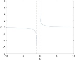
Created by Miao Yu
The shape of with respect to  can be found in fig. 9.2. It can be seen that Equation (9.7) satisfies the properties
(12) 
The property that  goes to infinity as the state approaches the boundary of the safe set makes it clear why the term “barrier” is used. Given Equation (9.7), one common idea to ensure the forward invariance of is to enforce
  . However, this is overly constrained as when the state is far from the boundary
  . Tthere is no need to constrain the barrier function to be non-increasing when the states are far from the boundary. One way to relax the condition is as following
(13) 
with positive  . In this way, when the state is far from the boundary of the safe set, Equation (9.9) allows the barrier function to grow. When the state approaches the boundary, i.e., when
  , we will have
  and thus force the changing rate to decrease to zero.
Another commonly used barrier function is
(14) 
It can be easily seen that Equation (9.10) also satisfies the properties in Equation (9.8). Plug Equation (9.10) into Equation (9.9), we can have the inequality
(15) 
From Equation (9.11), if  , i.e,
  , then
  , which means
  for all future time, thus guarantees the forward invariance of the safe set.
Equation (9.7) and (9.10) are two commonly used examples for reciprocal barrier functions. Next, we will provide a general definition of a reciprocal barrier function [9].
Definition 9.3
, a continuously differentiable function  is a reciprocal barrier function (RBF) for the set defined by Equation (9.4) and (9.5) for a continuously differentiable function
  , if there exist class
  functions
  such that, for all
  ,
,
Where a class function is defined as  with
with  and strictly increasing. Lie derivative is defined as
  .
.
From definition 9.3, since is bounded by two functions of the form  for some
  , the barrier function must behave like
  for some class function with the property
(17) 
Next, we will introduce a lemma that will be used to prove the theorem from [9], which describes the relation between RBF and the forward invariance of the safe set.
Lemma 9.1

 , the system has a unique solution defined for all
  and given by
 is a class
 In lemma 9.1, class  functions are continuous functions
  and for fixed
  ,
,  belongs to class , for fixed
  , the function is decreasing with respect to and
  as
as  .
.
Theorem 9.1
Given a set  defined by Equation (9.4) and (9.5) for a continuously differentiable function , if there exists a RBF , then
  is forward invariant.
Proof
Using Equation (9.12) and (9.13), we have that
(20) 
Since the inverse of a class function is a class function, and the composition of class function,  is a class function, [1].
Let  be a solution of with
  , and let
  . The next step is to apply the Comparison Lemma to Equation (9.17) so that
  is upper bounded by the solution of Equation (9.15). To do so, it must be noted that the hypothesis “
 is locally Lipschitz in ” used in the proof of Lemma 3.4 in [1], can be replaced by with the hypothesis “ is continuous, non-increasing in “. This is valid because the proof only uses the local Lipschitz assumption to obtain uniqueness of solutions to Equation (9.15), and this was taken care of with Peano’s Uniqueness Theorem in the proof of lemma 9.1 (not provided in this section, see [9]).\\
Hence, the Comparison Lemma in combination with lemma 9.1 yields
(21) 
for all  , where
  . This, coupled with the left inequality in Equation (9.12), implies that
(22) 
for all  . By the properties of class and functions, if
  and hence
  , it follows from Equation (9.19) that
  for all . Therefore,
  for all , which implies that is forward invariant.
Another form of barrier functions is called zeroing barrier functions. Due to the page limit, we will not introduce it in detail. The definition of extended class and zeroing barrier functions are as follows [1, 9].
Definition 9.4
A continous function  is said to belong to
  for some
  if it is strictly increasing and .
Definition 9.5
 with
with  such that, for all
  ,
,
9.3.3 Control Lyapunov Functions
Now that we have the barrier functions to verify the safety of a dynamical system, we can try to find a method that force the system to guarantee the safety. And this is a similar logic as in control Lyapunov functions (CLF). To motivate the safety-critical controller design, this section will first introduce one of the commonly used methods in state feedback sta-bilization design, control Lyapunov functions. Stabilization of equilibrium points is the core task in feedback control of nonlinear systems. Many techniques can be used to achieve this objective, e.g., partial feedback linearization, backstepping, passivity-based control, etc. [1]. Among these methods, CLF provides a systematic way to design the feedback controller, and the exis-tence of CLF is also a sufficient condition for the existence of a stabilizing state feedback control, which makes it a crucial technique. For detailed definitions and proofs shown in this section, see [1, 4].
Given a nonlinear system in the form of Equation (9.1), suppose the control objective is to stabilize the state to an equilibrium point  . Suppose there exists a locally Lipschitz stabilizing state feedback control
  such that the origin of
(24) 
is asymptotically stable. Then, by the converse Lyapunov theorem [1], there is a smooth Lyapunov function  such that
(25) 
where  are Lie derivatives
  ,
,  , respectively, and
  is a class function on the entire real line, i.e.,
  , and
, and  is strictly increasing. If such
  exists, it is called the control Lyapunov function. The corresponding can be applied to drive converge to the origin. Concretely, is a control Lyapunov function if it is positive definite and satisfies [4]
(26) ![\begin{equation*} \underset{\boldsymbol{u}\in U}{\text{inf}}[L_fV(\boldsymbol{x})+L_gV(\boldsymbol{x})k(\boldsymbol{x})]\leq-\gamma(V(\boldsymbol{x})). \quad\quad\quad(9.23)\nonumber \end{equation*}](https://opentextbooks.clemson.edu/app/uploads/quicklatex/quicklatex.com-a315a6443dd8b9de9f80333b263f3fed_l3.png "Rendered by QuickLaTeX.com")
Therefore, we can write the set that contains all stabilizing controllers for every point  as
as
(27) 
Note that if satisfies Equation (9.22), it must have the property
(28) 
Therefore, given a CLF , a stabilizing state feedback control is given by , where
(29) ![\begin{equation*} k(\boldsymbol{x}) = \begin{cases} -[L_fV+\sqrt{(L_fV)^2+(L_gV)^4}]/L_gV, &\text{if $L_gV\neq0$}\\ 0, &\text{if $L_gV=0$} \end{cases}\quad\quad\quad(9.26)\nonumber \end{equation*}](https://opentextbooks.clemson.edu/app/uploads/quicklatex/quicklatex.com-e3f572aa70e4ab96d0b0bf4af335d92f_l3.png "Rendered by QuickLaTeX.com")
To show that Equation (9.26) stabilizes the origin, we can choose V as the Lyapunov function candidate. Then, for  , if
, if  , from Equation (9.25), we have
(30) 
and if  , we have
(31) ![\begin{align*} \dot{V}&=\frac{\partial V}{\partial\boldsymbol{x}}(f(\boldsymbol{x})+g(\boldsymbol{x})k(\boldsymbol{x}))\nonumber\\ &=L_fV-[L_fV+\sqrt{(L_fV)^2+(L_gV)^4}]\nonumber\\ &=-\sqrt{(L_fV)^2+(L_gV)^4}\nonumber\\ &<0\nonumber \end{align*}](https://opentextbooks.clemson.edu/app/uploads/quicklatex/quicklatex.com-d72575aa3054230ecebeb5451b2d9433_l3.png "Rendered by QuickLaTeX.com")
Thus, for all  , in a neighborhood of the origin,
  , which shows that the origin is asymptotically stable. The following example will demostrate how CLF will be used in control design.
Example 9.3
Design a controller for the scalar system
(32) 
to stabilize the origin  .
.
One can use feedback linearization to stabilize the origin by choosing the control to be  ,
,  . The asymptotical stability can be proved by .\\
If we choose  as the control Lyapunov function, then by Equation (9.26), the control can be written as
(33) 
Figure 9.3 shows the comparison of the control $u$ and the closed-loop  between feedback linearization (
 ) and CLF. We can see that CLF results in a much smaller magnitude of the control for large
  , and meanwhile, much faster decaying rate for large . In this example, the control
  in CLF takes advantages of the nonlinear term
  , which is ignored by feedback linearization.


Figure 9.3: Comparison of the control  and the closed-loop between feedback linearization (red dashed curve) and CLF (blue solid curve).
Created by Miao Yu
The role of CLF in safety-critical control with barrier functions will be introduced in section 9.3.4. Furthermore, inspired by the idea of CLF, we can use similar method to ensure the system safety, which will be discussed in section 9.3.4.
9.3.4 Control Barrier Functions
Inspired by the idea of control Lyapunov functions, along with the fact that Lyapunov theorem can be used to verify the forward invariance of a superlevel set consist of Lyapunov functions (or Lyapunov-like functions), it is natural to extend this idea to safety critical systems with barrier functions.
In section 9.3.2, we introduced the concept of barrier functions for autonomous systems . Now we are ready to extend this idea into dynamical system in the form of Equation (9.1) to guide the safety-critical control design. Firstly, given that a reciprocal barrier function for an autonomous system needs to satisfy Equation (9.12) and (9.13) and it results in the property of Equation (9.14), what if cannot have the set to be forward invariant? How can we design a controller to ensure the forward invariance of  ? This leads to the following definition [9].
Definition 9.6
Consider the control system Equation (9.1) and the set defined by Equation (9.4) and (9.5) for a continuously differentiable function . A continuously differentiable function is called a reciprocal control barrier function (RCBF) if there exist class functions such that, for all  ,
,
(34) 
(35) ![\begin{equation*} \underset{\boldsymbol{u}\in U}{\text{inf}}[L_fB(\boldsymbol{x})+L_gB(\boldsymbol{x})\boldsymbol{u}-{\alpha_3(h(\boldsymbol{x}))}]\leq0. \quad\quad\quad(9.28)\nonumber \end{equation*}](https://opentextbooks.clemson.edu/app/uploads/quicklatex/quicklatex.com-f3ec9af4d02a1d5e94b98b590100e047_l3.png "Rendered by QuickLaTeX.com")
\noindent The RCBF is said to be locally lipschitz continuous if  and
and  are both locally Lipschitz continusous.
Guaranteed Safety via RCBFs. Note that definition 9.6 is the control system version of definition 9.3 by changing  to
to  . Now we can define the set that contains all the possible controllers that satisfy definition 9.6. For a given RCBF , for all ,
(36) 
When determining the control, if we choose the controller from the set  , it will allow us to guarantee the forward invariance of . This can be formally stated in the following corollary, which is a direct application of theorem 9.1, [9].
Corollary 9.1
Consider a set be defined by Equation (9.4) adn (9.5) and let be an associated RCBF for the system of the form in Equation (9.1). Then any locally lipschitz continuous controller  such that
  will render asymptotical the set forward invariant.
Similarly, based on the idea of ZBF (definition 9.5), we can have the definition of corresponding CBF.
Definition 9.7
 defined by Equation (9.4) and (9.5) for a continuously differentiable function
  function α such that for the control system Equation (9.1):
![\begin{equation*} \underset{\boldsymbol{u}\in U}{\text{sup}}[L_fh(\boldsymbol{x})+L_gh(\boldsymbol{x})\boldsymbol{u}]\geq -\alpha(h(\boldsymbol{x})), \quad\quad\quad(9.30)\nonumber \end{equation*}](https://opentextbooks.clemson.edu/app/uploads/quicklatex/quicklatex.com-3c7281db9009b7bc8ce081572e08fafd_l3.png "Rendered by QuickLaTeX.com")
Note that one of the major differences between ZBF and RBF is that RBF focuses on the forward invariance of the interior of safe set  , while ZBF focuses on the forward invariance of the entire safe set, . This is also true for ZCBF and RCBF.
Guaranteed Safety via ZCBFs. Therefore, similar as Equation (9.29), one can define the set that contains all the possible controllers that satisfy definition 9.7. For a given ZCBF ,
(38) 
Similar to corollary 9.1, the following result guarantees the forward invariance of , [4].
Corollary 9.2
Let be a set defined as the superlevel set of a continuously differentialble function  . If is a control barrier function on
  and
and  for all
  , then any Lipschitz continuous controller
  for the system Equation (9.1) renders the set safe. Additionally, the set is asymptotically stable in .
Corollary 9.2 states that the safe set is not only forward invariant, but also asymptotically stable under the controller . This means in the practical applications, system noise and uncertainties may force the system to enter the unsafe set. However, according to corollary 9.2, the controller is able to drive the system back to the safe set.
Necessity for Safety. Next, we will provide the lemma and theorem showing the necessity for barrier functions to safe set. The necessity for CBF will be a direct extension.
Lemma 9.2
Consider the dynamical system and a nonempty, compact set defined by Equation (9.4) and (9.5) for a continuously differentiable function . If  for all
  , then for each integer
  , there exists a constant
  such that
(39) 
Theorem 9.2
Under the assumptions of lemma 9.2,  is a RBF and
  is a ZBF for .
Proof
Let k = 3 in lemma 9.2. Then there exists  such that for all ,
  holds, which implies that
  holds, or equivalently,
  holds. By definition 9.3,
  is an RBF for .
The next corollary extends theorem 9.2 to CBF.
Corollary 9.3
Let be a compact set that is the superlevel set of a continuously differentiable function  with the property that
  for all . If there exists a control law that renders safe, i.e., is forward invariant with respect to
  , then
  is a control barrier function on .
9.3.5 Applications
Now that we have introduced the concepts and theorems of CBFs, we can finally start to discuss how CBF can be applied in the robotics field. In this part, we will introduce two optimization-based techniques that are used in robotics. Furthermore, we will briefly discuss some practical applications in advanced manufacturing.
Quadratic Optimization-Based CBF Control. As discussed in section 9.3.4, if we choose the controller from sets like Equation (9.31) and (9.29), we can guarantee that the set is forward invariant, i.e., safe. However, in most cases, there will be multiple (probably infinite many) feasible solutions for the controller that satisfy the CBF condition, in this case, we need to determine the “best” safe controller. Given the system Equation (9.1), suppose the desired controller without safety constraint is . To ensure safety, we need the controller to satisfy Equation (9.29) or Equation (9.31), and in the mean time, we want to make minimal changes to  . In this case, we define “best” as minimal 2-norm. This idea leads to the following quadratic programming (QP) problem (using ZCBF, RCBF is similar):
(40) 
CLF-CBF-Based Safety-Critical Control. As discussed in previous sections, CLF and CBF share very similar logic. Therefore, it is not a surprise that CBF can be added as an additional constraint in CLF-based control. In this way, one can achieve state feedback stablizatoin (or trajectory tracking) and meanwhile guarantee safety.
(41) 
where  is the weight matrix, and
  is a relaxation variable ensures the feasibility of the QP as penalized by
  .
.
Applications in Advanced Manufacturing and Robotics. One of the applications using CBF is adaptive cruise control for vehicles and mobile robots. By combining CLF and CBF, the system can track the desired velocity and in the mean time, guarantee the safety. In this context, safety can have different meanings, depend on the design purpose. For example, safety can mean “keep a safe distance from the car in front of you”, or “detour to avoid unexpected obstacles in the way”.
Another very insteresting application is ensuring safe walking for bipedal robots with precise footstep placement [5]. Footed robots have shown potentials over wheeled robots in many areas, such as navigation or searching in uneven terrain. In discontinued, unevern terrain (see fig. 9.4), only using CLF-based control with fixed trajectories cannot handle the task. Therefore, CLF-CBF-QP is introduced to guarantee precise foot placement for each step. It is worth noting that to define the foot placement in the safe set, [5] uses the method shown in fig. 9.5. The safe area for the next foot placement is displayed as bold red line in the figure. For each step, two circles are generated, each intersects with the end of safe area by one point, as shown in the figure. Then the safe set is defined as the area among two circles and the floor (the blue area in the figure). Along with CLF, the bipedal robot can thus achieve safe walking over uneven terrain.
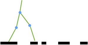
Created by Miao Yu based on information from [5].

Created by Miao Yu based on information from [5].
9.4 Hamilton-Jacobi Reachability Analysis (HJ-RA)
Hamilton-Jacobi reachability analysis is another important verification that is used to guarantee the performance and safety properties of dynamical systems [10, 11]. This section will briefly introduce the idea of backward reachable tube, backward reach-avoid tube, and how Hamilton-Jacobi equations can be used to determine the optimal controller under the worst-case disturbance.
9.4.1 Backward Reachable Tube (BRT)
First, we will introduce the concept of backward reachable set (BRS). This is the set of states such that the trajectories that start from this set can reach some given target set (see fig. 9.6). Here, if we define the target set to contain unsafe states, then the BRS is the set that the initial states should try to avoid.

Created by Miao Yu based on information from [10].
With the presence of the disturbance, we can treat the problem as a “Two Player Game” with Player 1 and Player 2 being the control input and system disturbance, respectively. Next, denote  as the target set wchich consists of the states that is known to be unsafe. Then, the role of Player 1 is to try to steer away from the target set with her input, while the role of Player 2 is to try to steer the system toward the target set with her input. Therefore, the BRS can be computed as
(42) )\in\mathcal{G}_0\},\,(9.35)\nonumber \end{equation*}](https://opentextbooks.clemson.edu/app/uploads/quicklatex/quicklatex.com-5b203c7b07a2549d507933310718673f_l3.png "Rendered by QuickLaTeX.com")
where ![\boldsymbol{\Gamma}[\cdot]](https://opentextbooks.clemson.edu/app/uploads/quicklatex/quicklatex.com-991cbc7e69e742c887c0b857c8a84211_l3.png "Rendered by QuickLaTeX.com") denotes the feasible set of strategies for Player 2.
denotes the feasible set of strategies for Player 2.
In reachability analysis, we assume Player 2 uses only non-anticipative strategies [10], i.e., Player 2 cannot have different responses to two Player one controls until they are different, which can be mathematically defined as
(43) ![\begin{equation*} \boldsymbol{\gamma}\in\boldsymbol{\Gamma}(t):=\{\mathcal{N}:U(t)\rightarrow D(t):\boldsymbol{u}(r)=\hat{\boldsymbol{u}}(r)\quad a.e. \quad r\in[t,s]\Rightarrow\mathcal{N}[\boldsymbol{u}](r)=\mathcal{N}[\hat{\boldsymbol{u}}](r) \quad a.e. \quad r\in[t,s]\}.\,(9.36)\nonumber \end{equation*}](https://opentextbooks.clemson.edu/app/uploads/quicklatex/quicklatex.com-68c67f99e9ff71f9cdb988293bed86c3_l3.png "Rendered by QuickLaTeX.com")
Additionally, Player 2 has the advantage of factoring Player 1’s choice of input and responding accordingly (instantaneous informational advantage). Therefore, the setup allows us to consider the problem in a worst-case scenario as Player 2 will respond to Player 1’s choice and try her best to steer the system to the target set (unsafe).
Equation (9.35) only gives “game of kind” instead of “game of degree” results, i.e., Equation (9.35) can only be used to determine whether or not the system states reaches the target set. Fortunately, we can use level set method to transform these games into games of degree. But before we introduce level set approach, we first need to introduce Hamilton-Jacobian Isaacs (HJI) that can be used to determine the optimal control from a cost function.
In many differential game problems as well as optimal control applications, the objective is to optimize (minimize or maximize) a cost function over the system trajectories and the final state. If we define  as the cost function during
 ![[t,0]](https://opentextbooks.clemson.edu/app/uploads/quicklatex/quicklatex.com-654882fe631f24f47f9c1d5f3808a4e6_l3.png "Rendered by QuickLaTeX.com") , then we can write it as
, then we can write it as
(44) 
where  denotes the cost at each time instant , and
  denotes the terminal cost. Then, in the “Two Player Game” setup, Player 1 will attemp to maximize the cost (steer away the target set) while Player 2 will attemp to minimize the cost (steer towards the target set). Therefore, under the assumptions to Player 1 and Player 2, the so-called “lower value” of the game can be written as
(45) 
where  is defined in Equation (9.36). In Equation (9.38),
  is used because we assume that Player 2 has the information of Player 1’s input choice and can respond accordingly.
From [12], Equation (9.38) is the viscosity solution of the HJI PDE
(46) 
where  is the Hamiltonian which is defined as
(47) 
where  is
is  and is called costate. Therefore, the optimal control for Player 1 can be obtained as [10]
(48) 
For more details, please see [12].
Going back to BRS in Equation (9.35), to convert it from “game of kind” to “game of degree”, it is always possible to define a Lipschitz function  based on the level set method such that the target set is the zero sublevel set of
  , i.e., we can have a Lipschitz function such that
  . If we define the cost function as
(49) 
then the system reaching the target set under control and disturbance is equivalent to  . Because, as discussed ealier, Player 1 wants to maximize the cost function, while Player 2 wants to minimize the cost function, and Player 2 has the instantaneous informational advantage, we can compute BRS using HBJ. Based on the discussion above, BRS can be defined as
(50) 
where  comes from Equation (9.38) and satisfies
(51) 
where the Hamiltonian is
(52) 
and the optimal control for Player 1 is
(53) 
To summarize, if  , then Player 1 can steer the system to avoid the target set, dispite Player 2’s input. Therefore, the reachability analysis provides a safety certificate as well as an optimal control solution with the presence of the system disturbance, which is one of the advantage of reachability analysis over control barrier functions.
Up till now, the BRS we discussed only cares about the states that starts exactly at time 0 and ends at time . Usually, a more practical problem is to check if a state can reach the target set within time duration  . This brings us the backward reachable tube (BRT), which can be similarly defined as [10]
(54) ![\begin{equation*} \mathcal{G}(t)=\{\boldsymbol{x}:\exists\boldsymbol{\gamma}\in\boldsymbol{\Gamma}(t),\forall \boldsymbol{u}\in U, \exists s\in [t,0], \,\zeta(s;\boldsymbol{x},t,\boldsymbol{u}(\cdot),\boldsymbol{\gamma}[\boldsymbol{u}](\cdot))\in\mathcal{G}_0\}.\quad\quad\quad(9.47)\nonumber \end{equation*}](https://opentextbooks.clemson.edu/app/uploads/quicklatex/quicklatex.com-29e1e304f3a64d137c0fb594ca823a55_l3.png "Rendered by QuickLaTeX.com")
9.4.2 Backward Reach-Avoid Tube (BRAT)
Similar to BRT, we can define another set that contains the initials states which have a control sequence that can drive the system towards the target set  (safe), dispite the worst-case disturbance, and in the mean time, avoid entering the unsafe set
  . This can be formally expressed as, [11]
(55) ![\begin{equation*} \mathcal{R}_{t_0}^{BRAT}(\mathcal{G},\mathcal{F}) = \{\boldsymbol{x}_0\in\mathcal{X}:\, \exists\boldsymbol{u}(\cdot),\forall\boldsymbol{d}(\cdot),\exists s\in[t_0,T], \zeta_{\boldsymbol{x}_0,t_0}^{\boldsymbol{u,d}}(s)\in\mathcal{G},\,\forall t\in[t_0,s],\zeta_{\boldsymbol{x}_0,t_0}^{\boldsymbol{u,d}}(t)\notin\mathcal{F}\}\,(9.48)\nonumber \end{equation*}](https://opentextbooks.clemson.edu/app/uploads/quicklatex/quicklatex.com-fc632fde073946babba944b13f369191_l3.png "Rendered by QuickLaTeX.com")
where similar as level set method in section 9.4.1, we can define the target set as  , and unsafe set as
  . Therefore, using the HJI, the optimal control law is given by
(56) 
where  is the value function
(57) ![\begin{equation*} \tilde{\mathcal{G}}(\boldsymbol{x},t) = \underset{\boldsymbol{u}}{\inf}\,\underset{\boldsymbol{d}}{\sup}\,\underset{t\in[t_0,T]}{\min}\max\{l(\zeta_{\boldsymbol{x},t_0}^{\boldsymbol{u,d}}(t)),\,\underset{s\in[t_0,t]}{\text{max}}\,g(\zeta_{\boldsymbol{x},t_0}^{\boldsymbol{u,d}}(s))\},\quad\quad\quad(9.50)\nonumber \end{equation*}](https://opentextbooks.clemson.edu/app/uploads/quicklatex/quicklatex.com-7a5ca8f9bb8bf8dc1399a71c60191d41_l3.png "Rendered by QuickLaTeX.com")
where the Hamiltonian is
(58) 
Finally, the BRAT-based controller can be defined as
(59) 
where  denotes the original desired controller, and
  is a small positive number provides the safety threshold.
9.4.3 Applications and Comparison to CBF
Now that we have introduced both CBF and reachability analysis, it is time to discuss their pros and cons, as well as the applications based on these properties. Note that this part will only discuss the advantages and limitations based on the classical problem setups. Given the rapid growth in safety-critical control area, researchers have been developing new techniques that aim to overcome the limitations of each method.
One of the major advantages of reachability analysis over CBF is that in the problem setup, HJ reachability analysis considers the presence of the disturbance or model uncertainty. Additionally, HJ reachability analysis treat the role of control input and disturbance as pursuer and evadar in a “two-player game”. Therefore, by finding the optimal control for HJ reachability analysis problem, one can find the optimal solution considering the worst-case scenario. The existence of the solution to the HJ reachability analysis indicates the existence of a control sequence that guarantees the system safety, dispite system disturbance. However, classical CBF does not consider the effect of the disturbance and could practically lead to unsafe configurations.
Another major difference between two methods is the computation complexity. Since HJ reachability analysis solves the PDE over grided state space using Dynamic programming, [11], its computation complexity increases expenontially with the number of system states. Therefore, classical HJ reachability analysis is usually stricted in applications with 4 or 5 states. Furthermore, due to the computation burden, HJ reachability analysis usually uses offline pre-computation. On the other hand, CBF converts the safety constraint into a simple linear constraint and thus can be easily solved by quadratic solver. Therefore, for applications that requires fast respond, e.g. walking robots, adaptive cruise control, etc, CBF is more applicable. Although HJ reachability analysis has the “curse of complexity”, researchers have developed various techniques, such as warm start and locally value function update technique, that significatly improves computation efficienty. These make HJ reachability analysis also applicable in some applications such as fast and safe tracking for motion planning, and unmanned aerial system traffic management, [10].
Last but not the least, developing a CBF might be challenging. There is no systematic way to construct a CBF for a system that is not feedback-linearizable [4]. Also, feasibility is another challenge in CBF based methods.
9.5 Summary
With the rapid development of the robotics, more and more applications are introduced in advanced manufacturing and daily life. This makes the safety bring more attention as autonomous are expected to operate in unkown environment, which makes it much harder to guarantee safety using conventional control methods. In this chapter, we discussed the concept of safety, and majorly introduced two commonly used safety-critical control methods, CBF and HJ reachability analysis. The chapter mainly focused on the problem derivation of two methods. Comparison between two methods and their applications were also briefly discusses. Finally, we will provide practice questions and simulation demostration using CBF techniques.
Practice Questions
Problem 1
What are the advantages and disadvantages of control barrier functions?
Advantages. Control barrier functions converts the safety constraint into a simple linear constraint and thus can be easily solved by quadratic solver. Therefore, CBF is capable of handling the applica-tions that require fast computation.
Disadvantages. There is no systematic way to construct a CBF for a system that is not feedback-linearizable. Besides, there might be no feasible solutions for a given CBF.
Problem 2
What are the advantages and disadvantages of reachability analysis?
Advantages. Reachability analysis considers the nonlinear problems with disturbance. Therefore, with proper definition of the disturbance, reachability analysis can provide the optimal controller that handles the worst-case scenario.
Disadvantages. The computation complexity increases exponentially with the number of states in reachability analysis. Therefore, the conventional reachability analysis can only be used in the nonlinear systems that has a maximum of four or five states.
Problem 3
Figure 9.7 is a 2D manipulator. Suppose that we want to steer the end-effector from the current position to the target (green dot in the figure). Since control is not the major topic in this chapter, we assume that the manipulator uses velocity control, i.e.,
(60) 
For now, we do not care about the obstacle.
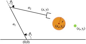
Created by Miao Yu
First, we need to compute the inverse kinematic for the configuration that the end-effector reaches the target. By assigning  , using the geometric method, we can write
(61) 
Here,  indicates the desired angle for each joint. Usually, there will be two solutions for this manipulator if the target is in the interior of the workspace. However, given the position of the target point, we need the configuration that stays above the floor. Thus, there is only one solution.
To steer the end-effector to the target, we can first define the error state ![\boldsymbol{e}=[e_1,e_2]^T](https://opentextbooks.clemson.edu/app/uploads/quicklatex/quicklatex.com-81f7e047a301fca3169131c96b3a0c65_l3.png "Rendered by QuickLaTeX.com") where
where
(62) 
and according to the system defined in the problem statement, we have
(63) 
Therefore, steering the end-effector to the target is equivalent to find a controller such that the error  will asymptotically approach to zero. One simple controller can be
(64) 
\noindent where  are positive numbers that controls the speed of convergence.
Problem 4
For the setup in problem 3, now we take the obstacle into consideration. Please define a safe set. To simplify the problem, we only consider the end-effector, i.e., we will allow the links to cross the obstacle if necessary.
First write the forward kinematics of the manipulator,
(65) 
\noindent Then to avoid the end-effector touching the obstacle, we need to ensure the distance between  and
and  to be larger than the radius , mathematically, we want
(66) 
Therefore, the safe set can be written as
(67) 
One can also write the safe set in terms of the system states  by replacing
  using forward kinematics. Additionally, the safe set only guarantees that the end-effector does not move across the obstacle. Usually, a “safer” way to define the safe set is to have the end-effector stays clear to the obstacle, i.e.,
(68) 
\noindent with some positive .
Problem 5
Use the safe set defined in problem 4, write a barrier function.
Note that there are multiple ways to define a barrier function. In this problem, we will use the reciprocal barrier function. Readers can also use zeroing barrier function introduced in this chapter as an exercise.
According to definition 9.3, we can define the barrier function as
(69) 
The above definition of the barrier function satisfies definition 9.3 by chosing
(70) 
Problem 6
Write a CBF-based safety-critical control using the barrier function defined in problem 5.
Denote the desired controller as  . We want to find a controller that guarantees the safety (collision avoidance), and in the mean time, have minimal change to . Thus, we have
(71) 
where we can choose  to be
to be  and
and
(72) ![\begin{align*} L_fh(\boldsymbol{\theta})+L_gh(\boldsymbol{\theta})\boldsymbol{u}=&0+\frac{1}{D^2}[-2(a_1c_1+a_2c_{12}-x_o)(-a_1s_1-a_2s_{12})+2(a_1s_1+a_2s_{12}-y_o)(a_1c_1+a_2c_{12})]u_1\\ &+\frac{1}{D^2}[-2(a_1c_1+a_2c_{12}-x_o)(-a_2s_{12})+2(a_1s_1+a_2s_{12}-y_o)(a_2c_{12})]u_2\\ D = &(a_1c_1+a_2c_{12}-x_o)^2+(a_1s_1+a_2s_{12}-y_o)^2,\nonumber \end{align*}](https://opentextbooks.clemson.edu/app/uploads/quicklatex/quicklatex.com-c0f24c8cc6e28aa1b660b4fd8b306cbe_l3.png "Rendered by QuickLaTeX.com")
where  denote
  , respectively, i.e.,
  , etc.
Simulation and Animation
In this part, we extend the manipulator problem into a 3-link case, see fig. 9.8. In the simulation, we set the green dot to be the target position, and the red ball to be the obstacle that the end-effector needs to avoid.

Created by Miao Yu
There are two cases in the simulation. The first case is the conventional control, and the second case is the conventional control with CBF as the constraint.
The simulation shows that the CBF-based safety-critical control can successfully steer the end-effector to the target point and meanwhile guarantees the collision avoidance.
References
[1] Hassan K Khalil. Nonlinear systems; 3rd ed. Prentice-Hall, Upper Saddle River, NJ, 2002.
[2] Charles Dawson, Sicun Gao, and Chuchu Fan. Safe control with learned certificates: A survey of neural lyapunov, barrier, and contraction methods. arXiv preprint arXiv:2202.11762, 2022.
[3] Hiroyasu Tsukamoto, Soon-Jo Chung, and Jean-Jaques E Slotine. Contraction theory for nonlinear stability analysis and learning-based control: A tutorial overview. Annual Reviews in Control, 52:135–169, 2021.
[4] Aaron D Ames, Samuel Coogan, Magnus Egerstedt, Gennaro Notomista, Koushil Sreenath, and Paulo Tabuada. Control barrier functions: Theory and applications. In 2019 18th European control conference (ECC), pages 3420–3431. IEEE, 2019.
[5] Quan Nguyen and Koushil Sreenath. Safety-critical control for dynamical bipedal walking with precise footstep placement. IFAC-PapersOnLine, 48(27):147–154, 2015.
[6] Mitio Nagumo. Uber die lage der integralkurven gew¨ohnlicher differentialgleichungen. Proceed-ings of the Physico-Mathematical Society of Japan. 3rd Series, 24:551–559, 1942.
[7] Stephen Prajna and Ali Jadbabaie. Safety verification of hybrid systems using barrier certificates. In HSCC, volume 2993, pages 477–492. Springer, 2004.
[8] Stephen Prajna. Barrier certificates for nonlinear model validation. Automatica, 42(1):117–126, 2006.
[9] Aaron D Ames, Xiangru Xu, Jessy W Grizzle, and Paulo Tabuada. Control barrier function based quadratic programs for safety critical systems. IEEE Transactions on Automatic Control, 62(8):3861–3876, 2016.
[10] Somil Bansal, Mo Chen, Sylvia Herbert, and Claire J Tomlin. Hamilton-jacobi reachability: A brief overview and recent advances. In 2017 IEEE 56th Annual Conference on Decision and Control (CDC), pages 2242–2253. IEEE, 2017.
[11] Zhichao Li. Comparison between safety methods control barrier function vs. reachability analysis. arXiv preprint arXiv:2106.13176, 2021.
[12] Lawrence C Evans and Panagiotis E Souganidis. Differential games and representation formulas for solutions of hamilton-jacobi-isaacs equations. Indiana University mathematics journal, 33(5):773–797, 1984.
