5 Dynamics
Joshua Norris
Chapter Outline
5.1 Newton-Euler Dynamics Review
5.2 Euler-Lagrange Dynamics
5.3 Summary
Practice Questions
Simulation and Animation
References
Introduction
A vital aspect of fully understanding and modeling the motion of a robot, whether that be a manipulator or a mobile robot, are its dynamics. The goal of dynamics is to create a mathematical model that is a representation of a rigid body's, in this case the robots, motion. This mathematical model is also called the robots equations of motion. These equations are a set of differential equations which can range from simple to extremely complicated. In many cases, certain assumptions or approximations are made that significantly reduce the complexity of the equations of motion. It's important to derive these equations of motion even if some approximations are to be made, since these equations can give an insight into the behavior of the robot. The equations can also be used to simulate the robot, which will be shown later in a simulation program.
In the field of dynamics there are multiple different methods to deriving the equations of motion for a rigid body. A very common one is the Newton-Euler method, also called Newton's method. This method is based on Newtons laws which were based on the dynamics of a particle. Later they were added onto by Euler, where he enhanced the original laws to apply to rigid bodies as well. Another popular method is called the Euler-Lagrange method, also called Lagrange's method. This method was generated cooperatively by both Euler and Lagrange and focuses more on the energy of the rigid body. Between the Newton method and the Lagrange method, the Lagrange method is much more applicable to the robotics being discussed in this book. However, the Newton method will still be given a review, as these two methods have a close relationship to each other. Thus, understanding the Newton method can give some insight into the Lagrange method. The Newton method is also the most commonly known and the most easily understood, so the review will aid in the understanding the Lagrange method later on in this chapter. If the topics of dynamics is of interest and the reader would like to go deeper with the knowledge, another more advanced method can be explored called the Hamiltonian method. [1] This method won't be covered, but it has a strong relationship with the Lagrange method, so it can be explored more after reading this chapter. A disclaimer for the rest of the chapter, in dynamics the generalized term "rigid body" is used a lot. In robotics, the rigid body that is being referred to depends on the robot itself. For a robotic manipulator the entirety of the system is a rigid body that can be analyzed as a whole, but the individual linkages are also rigid bodies that can be analyzed individually. For a manipulator, the linkages are coupled together, which means that the dynamics of each linkage will affect the other linkages, so the linkage dynamics must be analyzed in a holistic sense. In a mobile robot, it's usually the entire robot being analyzed as a rigid body, but individual parts of the mobile robot are technically rigid bodies as well. However, it can be redundant to analyze these individual parts.
5.1 Newton-Euler Dynamics Review [2]
As mentioned before, the Newton method is based on Newtons laws, specifically the second law. This law essentially states that the summation of forces is equal to mass multiplied by acceleration. Since robotic manipulators can move in 3 dimensional space, these summations apply to x, y, and z coordinates. The angular acceleration equation is based on the summation of moments about a specified point. These equations can be seen below as Equations (5.1) - (5.4).
[latex]\Sigma F_{x} = ma_{x}[/latex] (5.1)
[latex]\Sigma F_{y} = ma_{y}[/latex] (5.2)
[latex]\Sigma F_{z} = ma_{z}[/latex] (5.3)
[latex]\Sigma M = I\alpha[/latex] (5.4)
[latex]F_{y}[/latex], [latex]F_{x}[/latex], [latex]F_{x}[/latex] and are the forces in the [latex]y[/latex], [latex]x[/latex], and [latex]z[/latex] direction for the Cartesian coordinate system, and [latex]m[/latex] is the mass of the rigid body. [latex]a_{x}[/latex], [latex]a_{y}[/latex], and [latex]a_{z}[/latex] are the accelerations of the rigid body in the [latex]y[/latex], [latex]x[/latex], and [latex]z[/latex] direction. Other coordinate systems like the polar coordinate system can also be used. [latex]M[/latex] represents any moment or torque acting upon the rigid body, while [latex]I[/latex] is the rotational inertia about one of the rigid body's axes. [latex]\alpha[/latex] is the rigid body's angular acceleration. These equations combined can allow for multiple unknowns to be solved for. The procedure for this method involves creating a free body diagram where the forces and the motion of a single rigid body is analyzed and these equations applied. However, for some problems these equations aren't enough. To solve for this, this method also encompasses a couple other equations. These equations are the generalized kinematic equations, the equation due to the conservation of momentum, and the equation due to the conservation of energy. The generalized kinematic equations are Equation (5.5) and (5.6), while the conservation of energy equation is Equation (5.7).
[latex]\overrightarrow{v_{B}} = \overrightarrow{v_{A}} + \overrightarrow{v_{relative}} + \overrightarrow{\omega}\times\overrightarrow{r}[/latex] (5.5)
[latex]\overrightarrow{a_{B}} = \overrightarrow{a_{A}} + \overrightarrow{a_{relative}} + \overrightarrow{\alpha}\times\overrightarrow{r} - \omega^{2}\overrightarrow{r} + 2\omega\times\overrightarrow{v_{r}}[/latex] (5.6)
These kinematic equations are used to create relationships between variables that may not be given, which can be used as additional equations to solve for other unknowns. Many variables within these equations are vectors, which are denoted by the bar above the variable. That means that each equation can be expanded into various components dependent on the coordinate system used. These components are separated into their own equations to solve for any missing information. [latex]v_{A}[/latex] and [latex]v_{B}[/latex] are the velocities of two points on the rigid body, while [latex]v_{relative}[/latex] is another velocity that is only used if point B is moving along the rigid body as well. This also applies to [latex]a_{A}[/latex], [latex]a_{B}[/latex], and [latex]a_{relative}[/latex]. [latex]\alpha[/latex] is once again the angular acceleration, while [latex]\omega[/latex] is the angular velocity of the rigid body. r is the distance between points A and point B of the rigid body, which starts from point A. These equations can sometimes be confusing, especially the notation, but following the examples at the end of the section should bring some more understanding.
[latex]KE_{1} + PE_{1} = KE_{2} + PE_{2}[/latex] (5.7)
The kinetic energy (KE) for a robot will come from linear and angular motion, while the potential energy (PE) will come from mainly gravity but sometimes a spring. So a more generalized form of Equation 5.6 can be developed by plugging in the equations for each respective energy, which can be seen as Equation 5.8.
[latex]\frac{1}{2} mv_{1}^{2} + \frac{1}{2} I\omega_{1}^{2} + mgh + \frac{1}{2}k\Delta x^{2}= \frac{1}{2} mv_{2}^{2} + \frac{1}{2} I\omega_{2}^{2} + mgh + \frac{1}{2}k\Delta x^{2}[/latex] (5.8)
The first two terms on either side represent the kinetic energy, which are from both linear and angular motion. The last two terms on either side represent the potential energy, which are from the weight of the rigid body and a spring force. The ability to find the energies of a system is very important, not only in the Newton method, but also in the Lagrange method. This is a powerful equation that will be the base for all robotic dynamic problems, so make sure to practice finding the energies of various systems. The [latex]m[/latex] in the equation represents the mass of the rigid body. [latex]\omega[/latex] represents the angular speed, while [latex]v[/latex] represents the linear speed. [latex]h[/latex] is the distance from the center of mass of the rigid body to the datum with zero potential energy. In physics, this is usually the ground, such as in projectile motion. In robotics this reference plane can also be the ground such as in mobile robots, but it can also be the base of the robot such as in robotic manipulators. Just imagine letting go of the rigid body, when the body comes to rest, where would it be? The difference between this point and the point the body is at now is [latex]h[/latex]. [latex]k[/latex] is the spring constant of the spring, which is usually known. It is in units Newtons per meter. [latex]\Delta x[/latex] is the relative distance that the spring is compressed or extended. In the Newton method this equation acts similar to momentum, in that it can find some missing information, or relate together unknown variables to solve for another unknown. In the Lagrange method, this equation is utilized to it's full potential. [1]
With these equations known, an interesting connection in the Newton method itself can be shown, which also leads to some interesting connections to the Lagrange method. In the Newton method, the Newton's second law is the biggest player and used to find the equations of motion, however Newtons second law is also the derivative of kinetic energy. This can be shown by substituting the acceleration in newtons law with its derivative form and doing some mathematical manipulation. This is shown in Equation 5.9.
[latex]\overrightarrow{F} = m\overrightarrow{a} = m \overrightarrow{\frac{dv}{dt}} = m \frac{dv}{dx}\overrightarrow{\frac{dx}{dt}} = m \overrightarrow{v} \frac{dv}{dx}[/latex] (5.9)
The [latex]dx[/latex] can be moved to the left-hand side with the force and both sides can be integrated. The integral of force across a distance is work (W), while the integral of velocity across velocity is just a simple one variable integration. The final result is Equation 5.10.
[latex]W = \frac{1}{2}mv_{f}^{2} - \frac{1}{2}mv_{i}^{2} = \Delta KE[/latex] (5.10)
[latex]v_{f}[/latex] represents the final velocity of the rigid body, while [latex]v_{i}[/latex] represents the initial velocity of the rigid body. These equations show an interesting connection. So first, the equations of motion with the current information relies on needing to use a free body diagram and newtons law to find them, and second, newtons law has a direct relationship with the energy of the body. This poses the question: Can the equations of motion also be derived using energy? The answer is yes, and that's exactly what the Lagrange method does. This is helpful especially in robotic applications, as generating the necessary free body diagrams can take much time and can be prone to error. The Lagrange method will be delved into in the next section, but before reading on try the example given to test out the Newtonian method. As well as watch the attached video, it's very helpful in understanding the kinematics portion of Newtons method, which seems to be the hardest to grasp.
Newtonian Method Example:

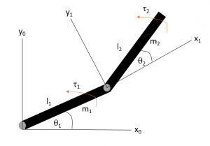
The linkages above have the masses [latex]m_{1}[/latex] and [latex]m_{2}[/latex]. Using Newtons method, find the equations of motion for the robotic manipulator.
Solution: Newtonian Method Solution
Video 5.1
5.2 Euler-Lagrange Dynamics [1][3]
As stated before, the Lagrange method is able to take the energy of the body/bodies and use that energy to find the equation(s) of motion. At first it seems daunting, however as examples are shown, it will be the preferred method. Especially in robotic applications. First, lets introduce the Lagrangian, which is the difference between the kinetic energy and the potential energy. This is shown as Equation 5.11.
[latex]L = T(q_{1}, q_{2},...,q_{n},\dot{q_{1}},\dot{q_{2}},...,\dot{q_{n}}) - V(q_{1},q_{2},...,q_{n}) = \Delta KE - \Delta PE[/latex] (5.11)
From here on out the sum of the kinetic energies will be represented by [latex]T[/latex], while the sum of potential energies is represented by [latex]V[/latex]. This is just to follow the conventions that are used in dynamics. The q's and [latex]\dot{q}'s[/latex] represent coordinates and are called generalized coordinates. This is another advantage for the Lagrange method, as it's equations can apply to any set of generalized coordinates. So, if a robot is moving across the floor in the [latex]x[/latex] direction only, the [latex]q[/latex] and [latex]\dot{q}'s[/latex] would be replaced with [latex]x[/latex] and [latex]\dot{x}[/latex]. However, this isn't the case for the robotic applications that are being looked at. The Lagrangian is the key in this method, and that is why knowing how to properly identify the energies is so important. From the Lagrangian, an equation can be derived. The derivation of this equation won't be shown here, however it's encouraged to research it or use the provided references [1] to read about it. The equation that is derived is Equation 5.12.
[latex]\frac{d}{dt}(\frac{\partial L}{\partial \dot{q_{i}}}) - \frac{\partial L}{\partial q_{i}} = 0[/latex] (5.12)
So, once the Lagrangian is found, take the partial derivative in respect to both the q and [latex]\dot{q}[/latex]. Once those are found, take a time derivative of the partial derivative that is in respect to [latex]\dot{q}[/latex]. That's all the information that is needed, at least for this form. This is the simplest form of the Lagrange equation, and is only valid for when there are only conservative forces. Once non-conservative and dissipative forces start to come into play the equation has to altered, however it still isn't too bad. For a non-conservative force a generalized force is used added onto the right hand side. This can be seen as equation 5.13.
[latex]\frac{d}{dt}(\frac{\partial L}{\partial \dot{q_{i}}}) - \frac{\partial L}{\partial q_{i}} = Q_{i} = \tau_{i}[/latex] (5.13)
An example for a non-conservative force would be a time-varying force. In robotic applications, this is usually an input torque which is why [latex]\tau_{i}[/latex] is shown in the equation. When dissipative forces are in the system, a term is added to the left hand side. This term is the derivative of the Rayleigh dissipation function in respect to [latex]\dot{q}[/latex]. The Rayleigh dissipation function, is a function of [latex]\dot{q}[/latex], and the damping coefficient, c. The Rayleigh dissipation function is equation 5.14.
[latex]F = \frac{1}{2}\sum_{i = 1}^{n}\sum_{j = 1}^{n} c_{ij}\dot{q_{i}}\dot{q_{j}}[/latex] (5.14)
This function represents a force such as a damping force caused by a damper. The [latex]b[/latex] is a damping coefficient, and the [latex]\dot{q}'s[/latex] are the derivatives of the generalized coordinates. These are summed to [latex]n[/latex], which represent all particles within a given system. When the derivative of this force is added into the Lagrange equation, Equation 5.15 is derived.
[latex]\frac{d}{dt}(\frac{\partial L}{\partial \dot{q_{i}}}) - \frac{\partial L}{\partial q_{i}} + \frac{\partial F}{\partial\dot{q_{i}}} = Q_{i} = \tau_{i}[/latex] (5.15)
This is the final form of the Lagrange equation, at least for the robotic applications that are being analyzed. The Lagrange equation can be taken even further as certain forces require Lagrange multipliers to be added into the equations, which involve analyzing constraint equations for the system. If the reader is interested in this, reference 1 delves deeper into the topic. However, this won't be talked about, but once again it's encouraged to research and read further into this if interested. With the Lagrange equation fully fleshed out try out the example below of a mass-spring-damper system.
Lagrange Method Example 1:

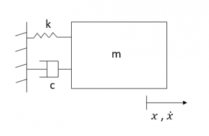
Using the Lagrange method, find the equation of motion of the above mass-spring-damper system.
Solution: Lagrange Method Solution 1
Applying the Lagrange method gets a bit more complicated, as now there are multiple rigid bodies all interacting with each other. The Jacobian will be used heavily, so make sure to review the previous kinematic chapters as needed.
For a robotic manipulator, a standard form for its equation of motion is normally used. This form is actually a standard form that can be used for other dynamic systems as well, under certain conditions. The first condition being that it's kinetic energy can be written in the form of equation 5.16.
[latex]K = \frac{1}{2}\dot{q^{T}}M(q)\dot{q}[/latex] (5.16)
[latex]M(q)[/latex] is the mass matrix, also sometimes written as [latex]D(q)[/latex] and referred to as the inertia matrix. If the kinetic energy can be written in this form, as well as if the potential energy is independent of [latex]\dot{q}[/latex], then the standard form can be used. For robotic manipulators both of these conditions are true, so the standard form can be used for them. The standard form is equation 5.17.
[latex]M(q)\ddot{q} + C(q,\dot{q})\dot{q} + g(q) = \tau[/latex] (5.17)
[latex]C(q,\dot{q})[/latex] is the Coriolis/centrifugal matrix, which doesn't always show up in the dynamics of the robots. It will most likely be in the dynamics of the robot that has a revolute joint. However, for a robot with only prismatic joints that are only producing linear motion, it won't show up. The [latex]g(q)[/latex] term is the gravitational force vector, which is related to the potential energy. Specifically, the terms come from the derivatives of the potential energy. Lastly, the [latex]\tau[/latex] is once again the input torque. The input torque is an important variable to know, as this input torque can actually be used to find the force at the end effector. Imagine a robotic manipulator doing a stamping or blanking manufacturing process. It's important to know everything that is happening at the end effector as it directly affects the product. Too much force and something could break. Too little force and the product is incomplete. The torque has a direct relationship to the end effector torque through the Jacobian. This relationship is equation 5.18.
[latex]\tau = J(q)^{T}f[/latex] (5.18)
The f represents the end effector force. The [latex]\tau[/latex] and the force will be a column vector, while the Jacobian will be a matrix.
The hardest part of this method is calculating the Coriolis/centrifugal matrix, and to do this Christoffel symbols are used. The equation to solve for the Christoffel symbols is equation 5.19.
[latex]c_{ijk} = \frac{1}{2}(\frac{\partial m_{kj}}{\partial q_{i}} + \frac{\partial m_{ki}}{\partial q_{j}} - \frac{\partial m_{ij}}{\partial q_{k}})[/latex] (5.19)
This equation seems long, but for the cases looked at in this book it can be simplified by saying: [latex]c_{ijk} = c_{jik}[/latex]. With the Christoffel symbols, each individual terms within the Coriolis/centrifugal matrix can be found. This is done using equation 5.20.
[latex]c_{kj} = \sum_{i = 1}^{n} c_{ijk}\dot{q_{i}}[/latex] (5.20)
The kth term will represent the rows of the C matrix, while the jth term will represent the columns of the C matrix. With all of this known, let's go back to a previous example done in the Newton method section, except this time with the Lagrange method.
Lagrange Method Example 2:

The linkages above have the masses [latex]m_{1}[/latex] and [latex]m_{2}[/latex]. Using Lagrange's method, find the equations of motion for the robotic manipulator.
Solution: Lagrange Method Solution 2
So here is step by step what exactly is happening in this solution. Firstly, the [latex]T[/latex] and [latex]V[/latex] were both found for the system. Next, the [latex]T[/latex] was plugged into equation 5.15, and used to solve for [latex]M(q)[/latex] or in this case [latex]D(q)[/latex]. With this mass/inertia matrix found, these can be used in equation 5.18 to find the Christoffel symbols. This in turn can be used in equation 5.19, to find the [latex]C(q, \dot{q})[/latex] matrix. With V already found, the partial derivative must be found in respect to each generalized coordinates, which gives the [latex]g(q)[/latex] matrix. Plug all of that into the standard form and those are the equations of motion. It's complicated still, but it's much easier than the Newtons method, especially with more complex robotic manipulators. These can also always be turned into a function in a program such as MATLAB or Python, so that it automatically generates all the matrices.
5.3 Summary
As engineers, scientists, or even hobbyists, knowing the dynamics of the robot in question is vital in controlling and using it properly. All the parts are interconnected together, so it can become very complex. Thankfully mathematical methods have allowed for a better understanding of this complexity and has simplified it tremendously. The Newton method, though not the best, is a great stepping stone to understanding motion and dynamics in general. Newtons laws completely changed how the world can be viewed, and allowed for the derivation of much better method, the Lagrange method. This method eliminates the strenuous efforts of creating free body diagrams for each individual rigid body, which is great for robotic manipulators and dynamics. With this method and modern technology, it's no longer a hassle to model the dynamics of systems. Hopefully, this chapter has provided a great recap/summary of dynamics and there application to robotics. Continue into the chapter to see how the ideas shown in this chapter can be applied to the modeling and simulation of robots.
Practice Questions
- Why are Euler-Lagrange dynamics preferred over Newton-Euler dynamics for robotic applications?
- What is the connection between the two methods?
- Why can the equations of motions of robotic manipulators be written in standard form?
- What are the three matrices used in the standard form?
- What are some real life situations where the information shown here can be used?
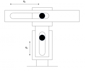
- What standard form matrix isn't in the solution for the problem below and why?
Simulation and Animation
The goal of the simulation is to confirm the validity of a set of equations of motion derived for a robotic manipulator. This robotic manipulator is the one seen in example 2 of the Lagrangian method section. The simulation software used are the python IDE, Spyder, as well as CoppeliaSim. Instead of making the simulation from scratch, the code and scenes are in a GitHub repository, which can be opened and used from the following link: https://github.com/ClemsonFall2021ME8930IntroRobotics-HRI/Ch5_Dynamics. The procedure for creating this simulation is also in the same link. To see the simulation ran and the results discussed further, please watch video 5.3, which is embedded below.
Video 5.3
References
[1] Greenwood, D. T., 1977, "Classical Dynamics" (1st ed.), Dover Publications, pp. 147-186
[2] Biggers, S.B., Orr, M.K., 2018, "Engineering Mechanics: Dynamics and Statics", McGraw Hill
[3] Spong, M. W., Hutchinson, S., & Vidyasagar, M., 2005, "Robot Modeling and Control" (1st ed.), Wiley, pp. 239-287


